Boosting Techniques in Machine Learning

Boosting Techniques in Machine Learning, in this Tutorial one can learn the Boosting algorithm introduction. Are you the one who is looking for the best platform which provides information about different types of boosting algorithm? Or the one who is looking forward to taking the advanced Data Science Certification Course from India’s Leading Data Science Training institute? Then you’ve landed on the Right Path.

Machine learning is vital for many of the technologies that seek to provide intelligence to the data, and companies recognize the great value. Boosting is a meta-algorithm joint learning machine to mainly reduce bias, and also variation in supervised learning, and a family of machine learning algorithms that convert students’ weaknesses to strengths.

The Below mentioned Tutorial will help to Understand the detailed information about boosting techniques in machine learning, so Just follow all the tutorials of India’s Leading Best Data Science Training institute in Bangalore and Be a Pro Data Scientist or Machine Learning Engineer.

Boosting Algorithm Introduction

As seen in the introduction part of ensemble methods, boosting is one of the advanced ensemble methods which improve overall performance by decreasing bias. Boosting is a consecutive process, where each succeeding model attempts to correct the errors of the preceding model.

Different Types of Boosting Algorithm

There are mainly five types of boosting techniques.

AdaBoost

Gradient Boosting (GBM)

Light GBM

XGBoost

CatBoost

Let’s see more about these types.

AdaBoost Algorithm in Machine Learning

Understanding AdaBoost Algorithm

AdaBoost, considered one of the simplest boosting algorithms, commonly utilizes decision trees for modeling. It follows a sequential approach, wherein multiple models are created successively. Each subsequent model aims to rectify the errors made by its predecessor.

This correction process involves assigning higher weights to observations that were incorrectly predicted by the previous model. Consequently, in the subsequent iteration, the algorithm prioritizes the accurate prediction of these misclassified instances. This iterative refinement of models ensures progressive improvement in overall prediction accuracy.

:

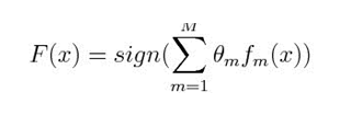
where

f_m = m^th weak classifier

_m= corresponding weight.

Understanding AdaBoost Algorithm

AdaBoost, short for Adaptive Boosting, is precisely the weighted combination of multiple weak classifiers. The algorithm operates through the following steps:

1. Equal Weight Initialization: Initially, all data points in the dataset are assigned equal weights.
2. Model Building: A subset of the data is utilized to build a weak model.
3. Prediction: Predictions are made for the entire dataset based on this model.
4. Error Measurement: Errors are evaluated by comparing the predictions with the actual values.
5. Weight Adjustment: Data points that are incorrectly predicted are assigned higher weights in the creation of the next model.
6. Weight Calculation: The weights for data points are determined based on the magnitude of errors. Higher errors correspond to higher weights for the respective data points.
7. Iterative Process: This process is repeated until either the error function stabilizes or the maximum limit of estimators is reached.

Let’s illustrate this process with an example of employee attrition.

Initializing and importing libraries

Import pandas as pd

Import numpy as np

Reading File

df=pd.read_csv(“Your File Path”)

df.head()

Splitting dataset into train and test

from sklearn.model_selection import train_test_split

train, test = train_test_split(df, test_size=0.3, random_state=0)

x_train=train.drop(‘status’,axis=1)

y_train=train[‘status’]

x_test=test.drop(‘status’,axis=1)

y_test=test[‘status’]

Applying AdaBoost:

from sklearn.ensemble import AdaBoostClassifier

model = AdaBoostClassifier(random_state=1)

model.fit(x_train, y_train)

model.score(x_test,y_test)

Output:

0.9995555555555555

Note: In the case of regression, the steps will be the same. Just we have to replace AdaBoostClassifier with AdaBoostRegressor.

 

Gradient Boosting (GBM) in Machine Learning:

Gradient Boosting, or GBM, represents an ensemble machine learning algorithm applicable to both regression and classification problems. GBM combines numerous weak learners to construct a robust algorithm. Similar to other boosting methods, each subsequent tree in GBM is built based on the error calculation from the preceding trees. In GBM, regression trees serve as the base learner.

Gender	Height	Weight	BMI	Physical Activity	Age
M	160	85	33.20	1	35
F	155	64	26.64	0	27
M	170.7	95	28.14	0	28
F	185.4	65	23.27	1	28
F	158	70	36.05	1	32
F	155	90	35.38	0	28
M	173.7	72	23.86	1	22
F	161.5	74	23.77	0	33

The mean age is supposed to be the predicted value (which is indicated by‘Predicition1’) for all observations in the dataset. The difference between mean age and actual values of age is considered as errors, which is indicated by ‘ Error 1’.

Prediction 1:

Gender	Height	Weight	BMI	Physical Activity	Age	Mean Age	Error
M	160	85	33.20	1	35	29	6
F	155	64	26.64	0	27	29	-2
M	170.7	95	28.14	0	28	29	-1
F	185.4	65	23.27	1	28	29	-1
F	158	70	36.05	1	32	29	3
F	155	90	35.38	0	28	29	-1
M	173.7	72	23.86	1	22	29	-7
F	161.5	74	23.77	0	33	29	4

Using Error 1 calculation, a tree model is designed. The purpose is to reduce that error to 0.

Prediction 2:

Gender	Physical Activity	Age	Mean Age(prediction 1)	Error1	Prediction 2	Mean + prediction 2
M	1	35	29	6	4	33
F	0	27	29	-2	-1	28
M	0	28	29	-1	-1	29
F	1	28	29	-1	0	29
F	1	32	29	3	1	30
F	0	28	29	-1	1	30
M	1	22	29	-7	-2	27
F	0	33	29	4	3	32

We will take the same example as the AdaBoosting technique. We will apply GBM on training and testing sets of the dataset.

from sklearn.ensemble import GradientBoostingClassifier

model= GradientBoostingClassifier(learning_rate=0.01,random_state=1)

model.fit(x_train, y_train)

model.score(x_test,y_test)

Output:

accuracy_score on test dataset :  0.7595555555555555

Note: In the case of regression, the steps will be the same. Just we have to replace GradientBoostingClassifier with GradientBoostingRegressor.

Light GBM Machine Learning:

Advantages of Light GBM for Large Datasets

When dealing with extremely large datasets, Light GBM emerges as a highly effective solution. This technique boasts superior speed when processing vast amounts of data compared to other algorithms. Unlike traditional level-wise approaches employed by certain algorithms, Light GBM utilizes a tree-based algorithm and adopts a leaf-wise approach.

Leaf-Wise Approach

In the leaf-wise approach, Light GBM constructs trees by splitting nodes based on the leaf that results in the maximum reduction of the loss function. This strategy enhances efficiency, particularly on large datasets, as it minimizes the number of levels in each tree.

However, it’s worth noting that the leaf-wise approach may lead to overfitting, especially on smaller datasets. To mitigate this risk, Light GBM provides a parameter called ‘max_depth’, which enables control over the maximum depth of each tree.

By leveraging these advantages and carefully tuning parameters like ‘max_depth’, Light GBM offers a powerful solution for handling large datasets efficiently while minimizing the risk of overfitting.

We will apply the Light GBM train data set and the model will predict for the test dataset.

First, install function

pip install lightgbm

Applying the algorithm to data sets

import lightgbm as lgb

train_data=lgb.Dataset(x_train,label=y_train)

#defining parameters

params = {‘learning_rate’:0.001}

model= lgb.train(params, train_data, 100)

y_pred=model.predict(x_test)

for i in range(0,4500):    # 4500 is number of datapoints iy_pred

if y_pred[i]>=0.5:

y_pred[i]=1

else:

y_pred[i]=0

# Accuracy Score on a test dataset

acc_test = accuracy_score(y_test,y_pred)

print(‘\naccuracy_score on test dataset : ‘, acc_test)

Output:

0.958

 

XGBoost in Machine Learning:

XGBoost, short for Extreme Gradient Boosting, represents one of the most advanced implementations of the gradient boosting algorithm. Renowned for its exceptional speed and high predictive power, XGBoost offers significant advantages over other boosting techniques. Its efficiency is evident, as it is nearly 10 times faster compared to its counterparts, making it a preferred choice for large-scale datasets.

Moreover, XGBoost addresses common issues such as overfitting by incorporating regularization techniques. By mitigating overfitting, XGBoost enhances the overall accuracy of the model, ensuring robust performance even on complex datasets. Its regularization properties have earned it the nickname ‘regularized boosting’ technique.

Now, let’s explore the application of the XGBoost technique on the same dataset to witness its effectiveness firsthand.

Import that library

pip install xgboost

Applying XGBoost on the next data set.

import xgboost as xgb

model=xgb.XGBClassifier(random_state=1,learning_rate=0.01)

model.fit(x_train, y_train)

model.score(x_test,y_test)

Output:

0.9995555555555555

CatBoost in Machine Learning:

It is difficult to handle large amounts of labeled data in case of the categorical values. Means if data is having many categorical variables then it is difficult to process the label encoding operation. In that case, ‘CatBoost’ can handle categorical variables and does not require extensive data preprocessing like other ML models. Let’s apply the technique to the same dataset.

Import library

 

pip install catboost

Applying CatBoost

from catboost import CatBoostClassifier

model=CatBoostClassifier()

categorical_features_indices = np.where(df.dtypes != np.float)[0]

model.fit(x_train,y_train,cat_features=([0,1,2,3,4]),eval_set=(x_test, y_test))

model.score(x_test,y_test)

Output:

0.9991111111111111

We hope you understand the boosting techniques in machine learning. Get success in your career as a Data Scientist by being a part of the Prwatech, India’s leading Data Science training institute in Bangalore.