Linear Regression
Linear Regression in Machine Learning
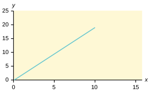
A linear equation with one independent variable is used in linear regression with two variables. The equation is written as y=a+bx, where a and b are both constants.
The independent variable is x, while the dependent variable is y. In most instances, you substitute a value for the independent variable before solving for the dependent variable.
Linear equations are used in the following cases.
y=3+2x y=–0.01+1.2x y=–0.01+1.2x
Learning Objectives
1. Explain what linear regression is.
2. Use a regression line to identify errors of estimation in a scatter plot.
We predict scores on one variable from scores on a second variable in simple linear regression. The criterion variable, also known as Y, is the variable we’re trying to forecast. The variable on which our forecasts are based is known as the predictor variable and is abbreviated as X. Easy regression is the prediction approach used where there is only one predictor variable. When the predictions of Y are plotted as a function of X in simple linear regression, which is the subject of this section, they form a straight line.
Figure 1 depicts the example data from Table 1. There is a good relationship between X and Y, as you can see. If you were to predict Y based on X, the higher the value of X, the more accurate your prediction of Y would be.
Table 1. Example data.
| X | Y |
| 1.00 | 1.00 |
| 2.00 | 2.00 |
| 3.00 | 1.30 |
| 4.00 | 3.75 |
| 5.00 | 2.25 |
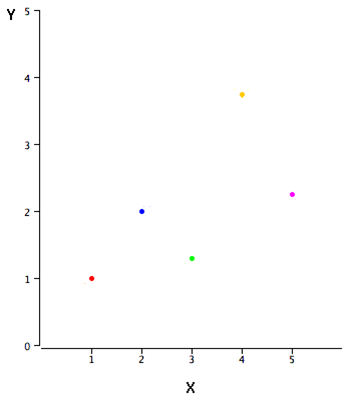
Figure 1. The example data in a scatter plot.
Finding the best-fitting straight line through the points is the objective of linear regression. A regression line is the best-fitting line. The regression line in Figure 2 is the black diagonal line that contains the expected Y score for each possible value of X. The errors of prediction are represent by the vertical lines connecting the points to the regression line. . The yellow point, on the other hand, is far higher than the regression line, and thus has a significant prediction
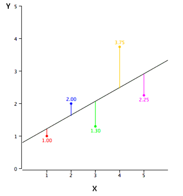
Figure 2. The example data in a scatter plot. The predictions are represented by the black line, the points by the actual data, and the vertical lines between the points and the black line by the prediction errors.
The value of the point minus the expected value is the prediction error for a point (the value on the line). Table 2 displays the forecast values (Y’) as well as the prediction errors (Y-Y’). The first point, for example, has a Y of 1.00 and a projected Y (referred to as Y’) of 1.21. As a result, its prediction error is -0.21.
Table 2. Example data.
| X | Y | Y’ | Y-Y’ | (Y-Y’)2 |
| 1.00 | 1.00 | 1.210 | -0.210 | 0.044 |
| 2.00 | 2.00 | 1.635 | 0.365 | 0.133 |
| 3.00 | 1.30 | 2.060 | -0.760 | 0.578 |
| 4.00 | 3.75 | 2.485 | 1.265 | 1.600 |
| 5.00 | 2.25 | 2.910 | -0.660 | 0.436 |
You may have noticed that we didn’t explain what “best-fitting rows” means. The line that minimizes the total of the squared errors of estimation is by far the most widely used criterion for the best-fitting line. The line in Figure 2 was discovered using this criteria. The squared errors of prediction are shown in the last column of Table 2. The sum of the prediction errors squared is lower than it would be for any other regression line, as shown in Table 2. A regression line’s formula is:
Y’ = bX + A
where Y’ denotes the predicted score, b denotes the line’s slope, and A denotes the Y intercept. The line in Figure 2 has the following equation:Y’ = 0.425X + 0.785
Computing the Regression Line:
The regression line is usually computed with statistical tools in the era of computers. The calculations, on the other hand, are reasonably simple and are provided here for anyone who is interested. The estimates are based on the Table 3 statistics. sX is the standard deviation of X, sY is the standard deviation of Y, MX is the mean of X, MY is the mean of Y, MX is the mean of X, MY is the mean of Y, MX is the mean of X, MY is the mean of Y, MX is the mean of X, MY
Linear Regression in Machine Learning