K Nearest Neighbors Algorithm Tutorial

When you move to a new city and look for a good restaurant, you do not study cuisine theory. You ask the people who live closest to you what they like. If most of your neighbours recommend the same place, you go there. The k nearest neighbors algorithm, usually shortened to KNN, makes predictions in exactly this way.

KNN is one of the simplest algorithms in machine learning. It has no training phase in the usual sense. It stores the data, and when a new point arrives, it finds the k closest points in the stored data and lets them decide. For classification, the neighbours vote for a class. For regression, their values are averaged. Because of this, KNN is called a lazy learner: it does no work until it has to predict.

In this tutorial, we explain how KNN works with a small picture example, then look at the three common ways of measuring distance, which are Euclidean, Manhattan and Hamming. We then cover the most important choice in KNN, the value of k, and why feature scaling can decide whether the algorithm works at all. A complete Python program follows, with output from a real run. We end with strengths, limitations, common mistakes and a short FAQ.

What is the K Nearest Neighbors Algorithm?

KNN is a supervised learning algorithm that predicts the label of a new point from the labels of its closest points in the training data. It makes no assumption about the shape of the data, which is why it is called non parametric. It has been used since the early days of pattern recognition and is still a handy first model, especially as a baseline.

The k in the name is the number of neighbours that get a vote. Its value is the main setting you control.

How does KNN Work?

Consider a plot with two groups of points, red stars and blue squares, and a new green circle whose class we do not know.

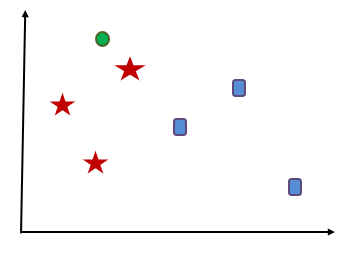
1. Choose k. Say k is 3.
2. Measure the distancefrom the green circle to every point in the data.
3. Pick the 3 nearest points.
4. Let them vote.If two of the three are red stars and one is a blue square, the circle is classified as a red star.

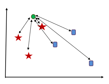
For regression, the last step changes. Instead of voting, the algorithm takes the average of the neighbours’ values.

Distance Measures Used in KNN

Everything in KNN depends on how distance is measured. Three measures are most common.

Euclidean Distance

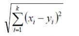
This is the straight line distance between two points, the one you would measure with a ruler. It is calculated by squaring the difference in each feature, adding the squares and taking the square root. It is the default for continuous numbers such as height, weight or temperature.

Manhattan Distance

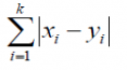
This is the distance you would travel in a city laid out in blocks, moving only along the grid. It adds up the absolute difference in each feature, without squaring. It is less affected by one very large difference, so it can work better when the data has outliers or many features.

Hamming Distance

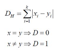
This is used for categorical data, such as colour or yes and no answers. It simply counts the number of features where the two points differ. If a feature matches, it adds 0. If it does not, it adds 1. For example, two records that agree on three of four categories have a Hamming distance of 1.

How to Choose the Value of K?

The value of k changes the result more than anything else.

• A small k, such as 1, follows the data very closely. It reacts to every noisy point, so it overfits. The decision boundary becomes jagged.
• A large ksmooths the boundary. If it is too large, it blurs real differences between classes and underfits.

A few practical rules help. For two class problems, choose an odd k, so votes cannot tie. Do not guess. Try a range of values and pick the one with the best score on data the model has not trained on. The usual tool is cross validation, which repeats the test on several splits so one lucky split does not decide.

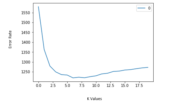
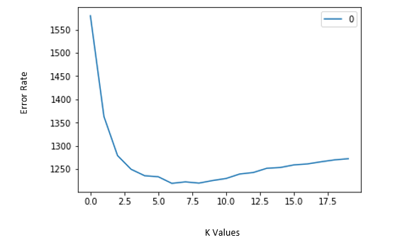
The classic way to see this is the elbow method. Plot the error rate for each k. The error often drops fast, then flattens. The point where it stops improving much is a good choice.

Why Feature Scaling Matters So Much?

Because KNN is based on distance, features with big numbers dominate. If one feature is income in rupees and another is age in years, a difference of 10,000 in income swamps a difference of 20 in age, and age is effectively ignored. Scaling puts every feature on a comparable range before distances are calculated. In the program below, the same model scores 0.722 without scaling and 0.963 with it, which is a very large jump from one line of preparation.

One more point is easy to get wrong. Fit the scaler on the training data only, and then apply it to the test data. If you fit the scaler on the test data as well, information from the test set leaks into the model, and your score becomes too optimistic.

KNN in Python With scikit learn

This program uses the Wine dataset that comes with scikit learn, which has 178 wines described by 13 chemical measurements and labelled with one of three types. It has three parts: a test of scaling, a search for the best k using cross validation, and a grid search over k, the distance measure and the voting style.

from sklearn.datasets import load_wine
from sklearn.model_selection import train_test_split, GridSearchCV, cross_val_score
from sklearn.neighbors import KNeighborsClassifier
from sklearn.pipeline import make_pipeline
from sklearn.preprocessing import StandardScaler

X, y = load_wine(return_X_y=True)
X_train, X_test, y_train, y_test = train_test_split(
    X, y, test_size=0.3, random_state=0, stratify=y
)

# Part 1: why scaling matters
raw = KNeighborsClassifier(n_neighbors=5).fit(X_train, y_train)
scaled = make_pipeline(StandardScaler(), KNeighborsClassifier(n_neighbors=5)).fit(X_train, y_train)
print("Without scaling:", round(raw.score(X_test, y_test), 3))
print("With scaling:   ", round(scaled.score(X_test, y_test), 3))

# Part 2: choosing k with cross validation on the training set
print("k  cv accuracy")
best_k, best = 1, 0
for k in range(1, 22, 2):
    model = make_pipeline(StandardScaler(), KNeighborsClassifier(n_neighbors=k))
    score = cross_val_score(model, X_train, y_train, cv=5).mean()
    print(k, round(score, 3))
    if score > best:
        best_k, best = k, score
print("Best k:", best_k)

# Part 3: grid search over k, distance metric and weighting
pipe = make_pipeline(StandardScaler(), KNeighborsClassifier())
grid = GridSearchCV(pipe, {
    "kneighborsclassifier__n_neighbors": [1, 3, 5, 7, 9, 11],
    "kneighborsclassifier__metric": ["euclidean", "manhattan"],
    "kneighborsclassifier__weights": ["uniform", "distance"],
}, cv=5)
grid.fit(X_train, y_train)
print("Best settings:", grid.best_params_)
print("Best cv accuracy:", round(grid.best_score_, 3))
print("Test accuracy:", round(grid.score(X_test, y_test), 3))

Without scaling: 0.722
With scaling:    0.963
k  cv accuracy
1 0.92
3 0.928
5 0.944
7 0.944
9 0.952
11 0.96
13 0.944
15 0.944
17 0.96
19 0.96
21 0.968
Best k: 21
Best settings: {'kneighborsclassifier__metric': 'manhattan', 'kneighborsclassifier__n_neighbors': 9, 'kneighborsclassifier__weights': 'distance'}
Best cv accuracy: 0.968
Test accuracy: 0.981

Part 1: The Effect of Scaling

When I ran the program, the first part printed:

Without scaling: 0.722
With scaling:    0.963

The test set has 54 wines, so that is 39 correct against 52 correct. The Wine data is a good example because one measurement, proline, runs into the hundreds while others are below 1. Without scaling, proline decides almost everything.

Part 2: Choosing k With Cross Validation

The second part tried the odd values of k from 1 to 21 using 5 fold cross validation on the training set:

k   cv accuracy
1   0.92
3   0.928
5   0.944
7   0.944
9   0.952
11  0.96
13  0.944
15  0.944
17  0.96
19  0.96
21  0.968

Best k: 21

• Very small k does worse.With k equal to 1 the score is 0.92, the lowest on the list, because one noisy neighbour decides.
• The scores then plateau.From k of 5 onward, results sit between 0.944 and 0.968.
• Do not over read the winner.The training set has only 124 wines, and the gap between k of 11 and k of 21 is about one wine. The best k landed on the edge of the range I tried, so a wider search could pick a different value. Treat k as anywhere on the plateau, not as a precise answer.

Part 3: Grid Search

The last part searched k, the distance measure and the weighting together. The weights setting decides whether every neighbour counts equally or closer neighbours count more:

Best settings: {'kneighborsclassifier__metric': 'manhattan', 'kneighborsclassifier__n_neighbors': 9, 'kneighborsclassifier__weights': 'distance'}
Best cv accuracy: 0.968
Test accuracy: 0.981

The grid search chose Manhattan distance, 9 neighbours and distance weighting, and scored 0.981 on the test set, or 53 of 54 wines. That is one wine better than the plain scaled model, so it is a small gain. It is a useful example of the method, and not proof that Manhattan beats Euclidean in general.

KNN for Regression

The original page uses a regression version, so here is how it differs. Use KNeighborsRegressor, which predicts the average of the k nearest values. Judge it with an error measure such as RMSE, the square root of the average squared error, and not with accuracy. The rules about scaling, choosing k and fitting the scaler on training data only stay exactly the same.

One caution applies to grid search. GridSearchCV uses the model’s default score, which for a regressor is R squared, not RMSE. If you want to choose k by RMSE, set the scoring option to neg_root_mean_squared_error. Otherwise the two methods can pick different values of k.

Strengths and Limitations of KNN

Strengths

• Easy to understand and explain.
• No training step, so new data can be added at any time.
• Works for both classification and regression.
• Makes no assumption about the shape of the data.
• A strong baseline to beat with more complex models.

Limitations

• Slow predictions on large data. Every prediction compares the new point with all stored points.
• Needs memory. The whole training set must be kept.
• Sensitive to scale. Unscaled features can ruin results.
• Struggles with many features. In very high dimensions, points all look about equally far apart, so neighbours stop meaning much. This is called the curse of dimensionality.
• Affected by noise and imbalanced classes. A common class can drown out a rare one.

Where KNN is Used?

• Recommendation systems. Suggesting products based on what similar customers bought.
• Document and text search. Finding documents closest to a query.
• Image recognition. Matching small images to known examples.
• Credit and risk scoring. Comparing an applicant to similar past cases.
• Missing value filling. Replacing a gap with the typical value among the nearest records.

Common Mistakes to Avoid

• Forgetting to scale. This is the number one KNN mistake, and the example above shows the cost.
• Fitting the scaler on the test data. It leaks information and inflates your score.
• Picking k by guess. Test a range with cross validation.
• Using an even k on a two class problem. Votes can tie.
• Using too many features. Remove features that carry no information.
• Using KNN on very large data without a plan. Prediction time will grow quickly.

KNN is simple, honest and easy to explain. It asks one question: who are your closest neighbours? Run the program above on your own data, scale before you measure distance, and choose k with cross validation. If predictions turn out too slow or accuracy plateaus, that is the time to look at models such as SVM or random forest.