Decision Tree Introduction with Examples
Decision Tree in Machine Learning: Introduction With Examples
Think about how a doctor narrows down a diagnosis. Is there a fever? If yes, is there a cough? If yes, is the oxygen level low? Each answer rules out some possibilities and points toward others, until a conclusion is left. A decision tree works the same way. It asks a chain of simple questions about your data, and each answer sends the case down one branch until it reaches a final answer.
Decision trees are among the easiest machine learning models to understand, because you can draw them and read them like a flowchart. They handle both classification, where the answer is a category, and regression, where the answer is a number. They need little data preparation, and they are the building block of random forests and boosting, two of the most successful methods for tables of data.
This tutorial explains how a decision tree works and how it decides which question to ask first. We cover the key terms, then the three measures that choose each split: entropy, information gain and Gini impurity. A worked example with every number calculated by running code makes it concrete. Then comes a complete Python program, run and checked, that shows a tree you can read, how depth causes overfitting, and how pruning fixes it. We finish with strengths, limits, common mistakes and an FAQ.
What is a Decision Tree?
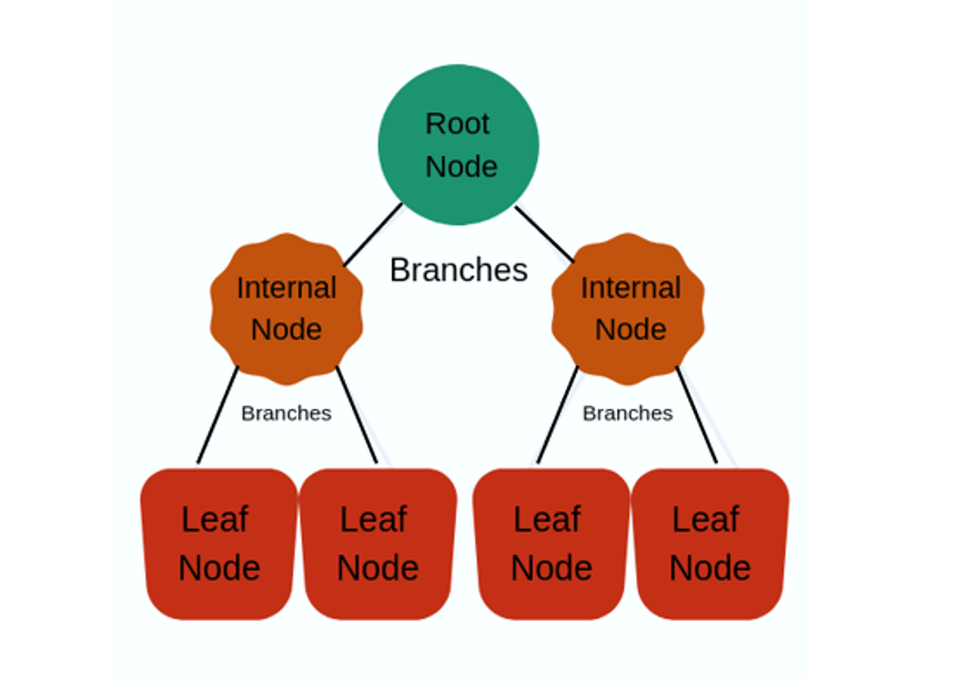
A decision tree is a supervised learning model that makes predictions by following a set of if then rules arranged as a tree. Each internal node tests one feature. Each branch is an outcome of that test. Each leaf at the end gives the final prediction, which is a class for classification and an average value for regression.
Common Terms Used With Decision Trees
| Term | Meaning |
|---|---|
| Root node | The top node, where the first split is made. It holds all the data |
| Splitting | Dividing a node into two or more sub nodes using a question |
| Decision node | A node that splits further into more nodes |
| Leaf or terminal node | A node that does not split. It gives the final answer |
| Branch or sub tree | A section of the tree |
| Parent and child node | A node that splits is the parent of the nodes it creates |
| Pruning | Removing branches to make the tree simpler and reduce overfitting |

The tree stops splitting a node when it is pure, or when no feature gives a gain above zero.
Gini Impurity
Gini impurity measures the chance that a randomly chosen item would be wrongly labelled if you labelled it at random, using the class proportions in the group. The formula is one minus the sum of the squared class proportions. A pure group scores 0. For two classes, an even mix scores 0.5, the worst case.
For the same group of 4 and 6, the proportions are 0.4 and 0.6. The Gini is 1 minus (0.16 plus 0.36), which is 0.48. Scikit learn uses Gini by default. It is a little faster to compute, and in practice it picks very similar splits to entropy.
| Measure | Pure group | Even two class mix | Group of 4 and 6 |
|---|---|---|---|
| Entropy | 0 | 1 | 0.971 |
| Gini impurity | 0 | 0.5 | 0.48 |
Decision Tree Example: Will We Play Cricket?
Here is a worked example with a complete table. Over 10 days, we noted the weather, humidity and wind, and whether the match was played. The values are made up to show the method.
| Day | Weather | Humidity | Wind | Play cricket |
|---|---|---|---|---|
| 1 | Sunny | High | Weak | No |
| 2 | Sunny | High | Strong | No |
| 3 | Cloudy | High | Weak | Yes |
| 4 | Rainy | High | Weak | Yes |
| 5 | Rainy | Normal | Weak | Yes |
| 6 | Rainy | Normal | Strong | No |
| 7 | Cloudy | Normal | Strong | Yes |
| 8 | Sunny | High | Weak | No |
| 9 | Sunny | Normal | Weak | Yes |
| 10 | Rainy | Normal | Weak | Yes |
Step 1: Entropy of the Whole Table
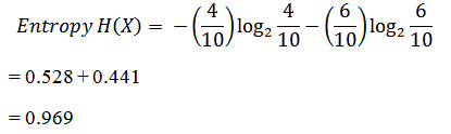
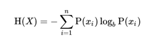
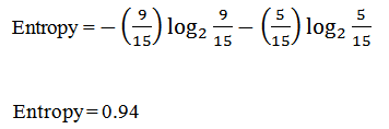
The match was played on 6 days and not played on 4. That is the same 4 and 6 split from before, so the entropy of the target is 0.971.

Where TT= Total number of targets=14
Step 2: Information Gain of Each Feature
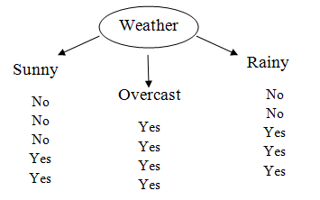
For each feature, we split the table by its values, calculate the entropy of each part, weight it by the share of rows, and subtract the total from 0.971. Here is the Weather feature:
| Weather | Days | Played | Entropy of the group |
|---|---|---|---|
| Cloudy | 2 | 2 | 0 (pure, always played) |
| Rainy | 4 | 3 | 0.811 |
| Sunny | 4 | 1 | 0.811 |
The weighted entropy is 0.2 times 0 plus 0.4 times 0.811 plus 0.4 times 0.811, which is 0.649. The gain is 0.971 minus 0.649, or 0.322. Note that the number 0.649 is the weighted entropy, which the original page loosely calls information.
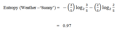
Here are the gains for all three features. I calculated these by running the code below.
| Feature | Weighted entropy | Information gain |
|---|---|---|
| Weather | 0.649 | 0.322 |
| Humidity | 0.846 | 0.125 |
| Wind | 0.880 | 0.091 |
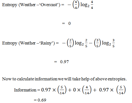
When I ran it, the key lines were:
Step 3: Choose the Root and Repeat
Weather has the highest gain at 0.322, so it becomes the root node. The Cloudy branch is already pure, since it always led to play, so it becomes a leaf that says yes. The Sunny and Rainy branches still hold a mix, so the algorithm repeats the process inside each one with the remaining features, Humidity and Wind, until the groups are pure or no gain is left. The finished tree looks like this.
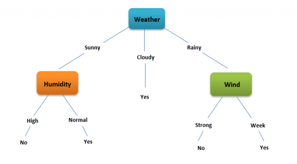
With only 10 rows, a deep tree would memorise the table and learn nothing general. This is a teaching example, and real trees need far more data.
Types of Decision Trees
- Classification treespredict a category, such as play or no play. Leaves hold a class, and splits are chosen with Gini or entropy.
- Regression treespredict a number, such as a house price. Leaves hold the average value of the rows in them, and splits are chosen to reduce the squared error.
CART, short for classification and regression trees, is the name of the overall method. It covers both types and always splits into two branches. It is the version scikit learn uses.
Overfitting and Pruning
A tree left to grow without limit keeps splitting until every leaf is pure. It then fits its training data perfectly, noise included, and fails on new data. This is overfitting, and it is the main weakness of decision trees. Pruning fixes it by cutting back branches that add little. There are two ways:
- Pre pruning.Stop early, using limits such as maximum depth or a minimum number of rows in a leaf.
- Post pruning.Grow the full tree, then cut back the weakest branches. Scikit learn does this with the ccp_alpha setting. A larger value prunes more.
Decision Tree in Python With scikit learn
This program has three parts. First it trains a small tree on the Iris flower dataset and prints it as readable rules. Then it uses the breast cancer dataset, with 569 patients and 30 measurements each, to show how depth and pruning change the result. Last it compares Gini with entropy. Both datasets come with scikit learn, so there is no file to load.
Part 1: A Tree You Can Read
Two questions about petal width are enough to separate three species. Anyone can follow these rules without knowing any statistics, which is the great strength of a tree. The test set has 45 flowers, so 0.956 means 43 correct.
Part 2: Depth and Overfitting
- Training accuracy keeps climbing. It reaches 1.0 at depth 8, which means the tree has memorised the training set.
- Test accuracy stops improving. It peaks at 0.93 for depth 5, then falls back to 0.918.
- Mind the small differences. The test set has 171 patients, and one patient is worth about 0.6 points. The gap between 0.918 and 0.93 is two patients, so treat it as a rough sign, not a precise answer.
- The tree stopped growing at 16 leaves. Depth 8 and no limit gave the same tree, because every leaf was already pure.
Part 3: Pruning
A small amount of pruning, with ccp_alpha at 0.005, cut the tree from 16 leaves to 7 and raised test accuracy from 0.918 to 0.93. That is a simpler tree that does the same job or a little better. Prune too hard, as at 0.02, and the tree becomes too simple and the score drops.
Part 4: Gini Against Entropy
On this data and this split, entropy scored 0.947 and Gini 0.924, a difference of about 4 patients out of 171. That does not prove one is better. In practice the two usually pick very similar trees, so do not spend time on this choice before tuning depth and pruning.
Advantages and Disadvantages of Decision Trees
Advantages
- Easy to understand and explain, and you can draw them.
- Handle both classification and regression.
- Need little data preparation. They do not need scaling.
- Handle numbers and categories, and capture curved and interacting patterns.
- Fairly robust to outliers, because splits depend on order, not on how extreme a value is.
Disadvantages
- Overfit easily if left to grow, which is the biggest weakness.
- A small change in the data can produce a very different tree.
- Predictions are steps, not smooth curves, which is a limit for regression.
- Biased toward features with many distinct values.
- Usually less accurate than random forests or boosting, which combine many trees.
Where Decision Trees Are Used
- Approving or rejecting loan applications with rules that can be explained.
- Triage and diagnosis support.
- Deciding which customers to target.
- Spotting faults from machine readings.
- Inside other models. Random forests and boosting are built from many trees.
Common Mistakes to Avoid
- Training and scoring on the same data. Always score on a held out test set.
- Leaving the depth unlimited. Set max_depth or use pruning.
- Trusting one tree.cCheck with cross validation or move to a random forest.
- Reading too much into a tiny example.cA tree trained on 10 rows teaches the method, not a real result.
- Mixing up entropy and information gain.cEntropy is the uncertainty. Gain is how much a split reduces it.
- Using a regression tree for a category or the reverse.cMatch the tree type to the target.
A decision tree turns data into a set of questions that anyone can follow. Learn how entropy, information gain and Gini choose each split, limit the depth or prune to avoid overfitting, and always judge the tree on data it has not seen. Once you are comfortable with one tree, move on to random forest and boosting, which use many trees to get higher accuracy.
