Random Forest Tutorial for Beginners

Suppose you want a second opinion on a medical report. You would not trust one doctor if you could ask a hundred, each trained a little differently and each looking at different details. If most of them reach the same conclusion, you can be fairly confident. A random forest works on this principle. It is a crowd of decision trees that vote.

Random forest is one of the most widely used algorithms in machine learning, and for good reason. It handles both classification and regression, works well with little tuning, copes with many features and gives you a measure of which features matter. It is often the first strong model people try on a table of data, and the one other models are compared against.

In this tutorial, we begin with the decision tree, the building block of the forest, and see why a single tree is not enough. We then explain how a random forest is built, how its trees split data using the Gini index, entropy or mean squared error, and what its strengths and weaknesses are. A complete Python program follows, with output from a real run that includes accuracy, precision and recall, the effect of the number of trees and the most important features. We finish with common mistakes and a short FAQ.

Random Forest in Machine Learning

Classification is a supervised learning task. The model learns from examples that already have labels, then predicts the label of new data, such as spam or not spam, or benign or malignant. Many algorithms do this, including logistic regression, KNN, SVM and Naive Bayes. Random forest is one of the strongest general purpose choices among them, and it is also used for regression, where the answer is a number and not a class.

Decision Tree: The Building Block of a Random Forest

A decision tree classifies data by asking a series of yes or no questions. Each question splits the data into smaller groups, and the final group gives the answer. For example, a tree for loan approval might ask whether income is above a limit, then whether there is a past default, and then end at approve or reject.

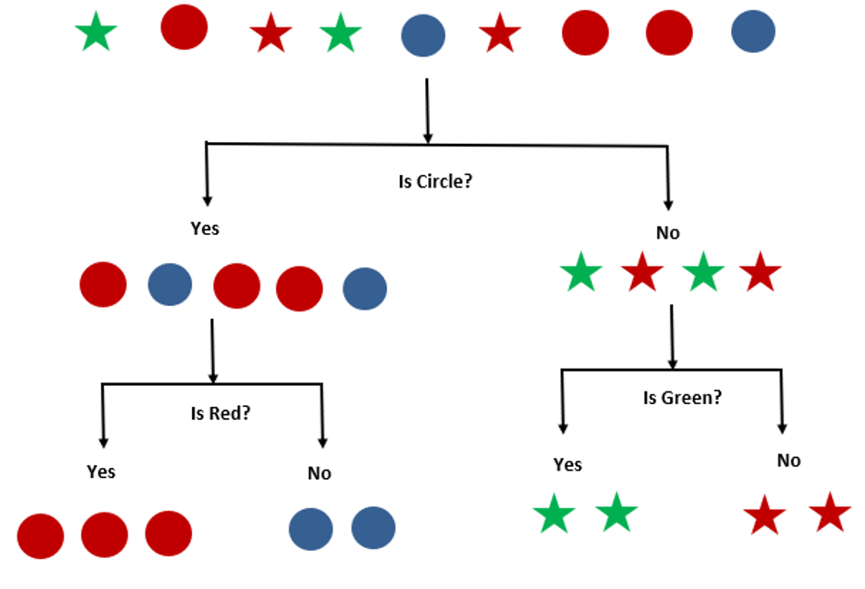
A single tree is easy to read, but it has a weakness. If left to grow deep, it memorises its training data, including the noise. Change a few rows and you can get a very different tree. That sensitivity is called high variance, and it is what the forest fixes.

What is a Random Forest?

A random forest builds many decision trees and combines their answers. Two kinds of randomness make the trees different from each other:

• Random rows.Each tree trains on a bootstrap sample, which is a random draw of rows with replacement. This is the bagging idea.
• Random features.At each split, a tree considers only a random subset of the features, not all of them. This stops every tree from relying on the same strong feature.

To predict, every tree gives its answer. For classification, the class with the most votes wins. In scikit learn, the forest averages the trees’ predicted probabilities, which usually gives the same answer. For regression, it averages the trees’ numbers.

Say a forest has 6 trees, and 4 of them predict class A while 2 predict class B. The forest answers class A. Even if two of the trees are wrong, the group is still right.

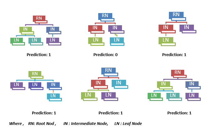
1. Draw a bootstrap sample of the training rows for each tree.
2. Grow a tree on that sample. At every split, look at only a random subset of features and pick the best split among them.
3. Repeat until you have the number of trees you want, 100 or more is typical.
4. Combine the trees. Vote for classification, average for regression.

Why is Random Forest Better Than a Single Tree?

Each tree makes its own mistakes, but because the trees are different, the mistakes point in different directions and largely cancel when averaged. The pattern that every tree shares is kept. The result is a model with lower variance than one tree, and usually higher accuracy on new data, without much extra effort.

How a Tree Chooses Its Splits?

At every node, a tree looks for the question that separates the data best. How it measures best depends on the task.

Regression: Mean Squared Error

For regression, a common choice is mean squared error, or MSE. It is the average of the squared gaps between the predicted values and the actual values. In the formula, N is the number of data points, fi is the value the model returns, and yi is the actual value for that data point. A split is chosen if it makes this error smaller. MSE is a common choice, not the only one.

Classification: Gini Index and Entropy

For classification, the tree uses a measure of how mixed the classes are in a node. A node with only one class is pure, and a node with an even mix is as impure as it gets. A good split makes the groups after the split purer than before.

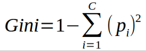
The Gini index is one minus the sum of the squared class proportions. In the formula, pi is the relative frequency of each class and c is the number of classes. It measures impurity. It does not measure which branch is more likely.

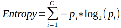
Entropy is another measure of impurity. It is the negative sum of each class proportion times the base 2 logarithm of that proportion.

Here is a worked example. A node holds 10 records, 6 of one class and 4 of the other, so the proportions are 0.6 and 0.4.

A perfectly even node would score 0.5 on Gini and 1 on entropy, so this node is quite mixed. In practice, Gini and entropy usually pick very similar splits. Gini is the default in scikit learn and is a little faster.

Random Forest in Python With scikit learn

This program uses the breast cancer dataset that comes with scikit learn, with 569 patients and 30 measurements each, labelled malignant or benign. It compares one tree with a forest, shows precision and recall, tests how the number of trees matters, lists the most important features and checks the Gini and entropy example above.

import numpy as np
from sklearn.datasets import load_breast_cancer
from sklearn.ensemble import RandomForestClassifier
from sklearn.metrics import accuracy_score, classification_report
from sklearn.model_selection import train_test_split
from sklearn.tree import DecisionTreeClassifier

data = load_breast_cancer()
X, y = data.data, data.target
X_train, X_test, y_train, y_test = train_test_split(
    X, y, test_size=0.3, random_state=42, stratify=y
)

# One tree against a forest
tree = DecisionTreeClassifier(random_state=42).fit(X_train, y_train)
forest = RandomForestClassifier(n_estimators=200, oob_score=True, random_state=42)
forest.fit(X_train, y_train)
print("Single tree accuracy:", round(tree.score(X_test, y_test), 3))
print("Forest accuracy:", round(accuracy_score(y_test, forest.predict(X_test)), 3))
print("Forest out of bag score:", round(forest.oob_score_, 3))

# Precision and recall, not accuracy alone
print(classification_report(y_test, forest.predict(X_test), target_names=data.target_names))

# How the number of trees changes the score
for n in [1, 10, 50, 200]:
    m = RandomForestClassifier(n_estimators=n, random_state=42).fit(X_train, y_train)
    print(n, "trees:", round(m.score(X_test, y_test), 3))

# The five most important features
order = np.argsort(forest.feature_importances_)[::-1][:5]
for i in order:
    print(data.feature_names[i], round(forest.feature_importances_[i], 3))

# Gini and entropy for a node with 6 of one class and 4 of the other
p = np.array([0.6, 0.4])
print("Gini:", round(1 - (p ** 2).sum(), 3))
print("Entropy:", round(-(p * np.log2(p)).sum(), 3))

Single tree accuracy: 0.918
Forest accuracy: 0.942
Forest out of bag score: 0.967
              precision    recall  f1-score   support

   malignant       0.94      0.91      0.92        64
      benign       0.94      0.96      0.95       107

    accuracy                           0.94       171
   macro avg       0.94      0.93      0.94       171
weighted avg       0.94      0.94      0.94       171

1 trees: 0.912
10 trees: 0.93
50 trees: 0.924
200 trees: 0.942
worst perimeter 0.141
worst area 0.132
worst concave points 0.122
worst radius 0.085
mean concave points 0.077
Gini: 0.48
Entropy: 0.971

Part 1: One Tree Against a Forest

When I ran the program, it printed:

Single tree accuracy: 0.918
Forest accuracy: 0.942
Forest out of bag score: 0.967

The test set has 171 patients, so the forest got about 4 more patients right than the single tree. The out of bag score is a free validation estimate, computed from the rows each tree did not see. It came to 0.967 without touching the test set.

Part 2: Accuracy Is Not Enough

              precision    recall  f1-score   support

   malignant       0.94      0.91      0.92        64
      benign       0.94      0.96      0.95       107

    accuracy                           0.94       171

Overall accuracy looks fine at 0.94, but look at the malignant row. Its recall is 0.91, which means the forest caught 58 of 64 malignant cases and missed 6. In a medical setting, a missed malignant case is the costly error, so recall for that class matters more than the headline number. This is the check the original page left out.

Part 3: How Many Trees?

1 trees: 0.912
10 trees: 0.93
50 trees: 0.924
200 trees: 0.942

One tree scores 0.912, and more trees help overall. But 50 trees scored a little below 10 trees, which is normal noise on a small test set, since one patient is worth about 0.6 points. The honest lesson is that more trees give steadier results, with diminishing returns. A forest does not get worse from adding trees. It only gets slower.

Part 4: Feature Importance

worst perimeter         0.141
worst area              0.132
worst concave points    0.122
worst radius            0.085
mean concave points     0.077

A forest can rank which features it relied on. Here the largest tumour measurements matter most. Treat this ranking with care. Perimeter, area and radius are strongly related to each other, so the forest splits the credit between them. The importance scores show what the model used, not what causes the result.

Important Settings of RandomForestClassifier

Advantages and Disadvantages of Random Forest

Advantages

• Works for both classification and regression.
• Reduces the overfitting of a single tree.
• Works well with default settings and little tuning.
• Handles many features and does not need feature scaling.
• Trees train independently, so training can run in parallel.
• Gives feature importance and an out of bag score.

Disadvantages

• Harder to interpret than one tree.
• Uses more memory and takes longer to predict with many deep trees.
• Cannot predict values outside the range it saw in training, which matters for regression on trends.
• Can still overfit noisy data, especially with unlimited depth.
• Feature importance can mislead when features are related to each other.

Where Random Forest is Used?

• Credit scoring and fraud detection.
• Disease risk from patient measurements.
• E commerce. Customer churn and product recommendation.
• Predicting equipment failure from sensor readings.
• Predicting prices and default risk.

Common Mistakes to Avoid

• Trusting accuracy alone. Check precision and recall, especially with imbalanced classes.
• Judging by training accuracy. A forest of deep trees will score near perfect on its own training data.
• Reading feature importance as cause. It shows what the model used.
• Using too few trees. Start with 100 or more.
• Leaving trees unlimited on noisy data. Set max_depth or min_samples_leaf.
• Forgetting random_state. Without it, results change each run.

A random forest turns many unstable trees into one dependable model. Run the program above on your own data, look at recall as well as accuracy, and use the out of bag score as a quick check. When you want to push accuracy higher, look at boosting next.