Regression Analysis Tutorial With Examples

How much will a flat of 1,500 square feet cost in your city? How many units will a shop sell next month if it spends more on stock? How much will a patient’s blood sugar change in a year? Each of these questions asks for a number, and each can be answered by looking at how one thing changes when another changes. That is what regression analysis does.

Regression analysis is one of the oldest and most useful tools in statistics and machine learning. It finds the relationship between an outcome you want to predict and the factors that influence it, and it turns that relationship into a formula you can use. It tells you which factors matter, how strongly, and what to expect when they change. Banks, hospitals, retailers and factories use it every day.

This tutorial explains regression analysis from the start. We cover what it is, why we use it, and the main types, then go deep on linear regression, the simplest and most common kind. Two worked Python examples follow, one with a single input and one with three. After them comes a proper test on data the model has not seen, with the right measures of error. We end with assumptions, common mistakes and a short FAQ.

What is Regression Analysis?

Regression analysis is a method that studies how a dependent variable, the outcome you want to predict, depends on one or more independent variables, the inputs that influence it. It builds a model linking them, and the model predicts the average value of the outcome for given inputs.

For example, the price of a house is the dependent variable. Its area, number of bedrooms and age are the independent variables.

Why do We Need Regression Analysis?

Regression helps in two ways. It shows which variables matter and how much, and it predicts outcomes for new cases.

• Finding what matters. Does gender affect salary after allowing for experience? Which factors push up a household’s water use?
• What is the likely price of a house, the sales for next month, or the demand for power on a hot day?
• Measuring strength. How closely are two things related, and is the link positive or negative?
• Testing ideas. Does an extra rupee of marketing really lead to extra sales?

Take household water use. Use depends on the number of people, the size of the home, the season and whether there is a garden. Regression estimates how much each of these adds, so a water utility can plan supply.

What Questions does Regression Answer?

• Is there a relationship between the variables?
• How strong is it?
• Is it positive, where both rise together or negative, where one rises as the other falls?
• How much does the outcome change for each unit change in an input?
• What outcome should we expect for a new case?

Types of Regression Analysis

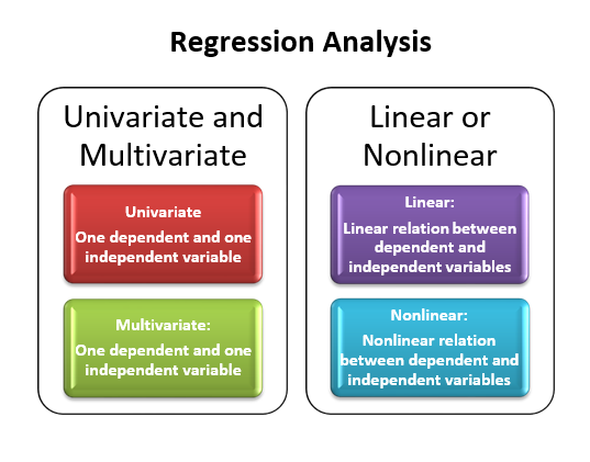
Regression comes in several forms, depending on the number of inputs and the shape of the relationship.

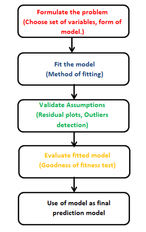
Building a regression model is a cycle. You fit a model, check how well it does on data it has not seen, and then improve it by adding or removing inputs, or by changing the type. Several rounds are normal.

Introduction to Linear Regression

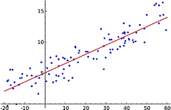
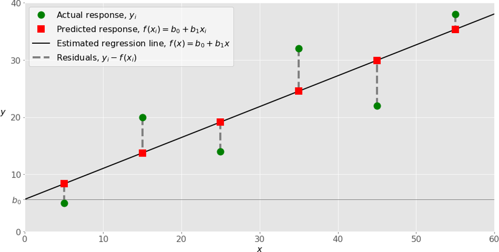
Linear regression fits a straight line through your data. The line has an equation you may remember from school: y = mx + c.

• y is the dependent variable, the thing we predict.
• x is the independent variable, the input.
• m is the slope, or coefficient. It is how much y changes for each unit increase in x.
• cis the intercept, the value of y when x is zero.

The line chosen is the best fit line. It is the one that makes the total of the squared gaps between the actual points and the line as small as possible. This method is called least squares.

A slope above zero means the two variables rise together, which is a positive relationship. A slope below zero means one falls as the other rises, which is a negative relationship. These describe the slope. They are not separate types of regression.

Types of Linear Regression

Simple Linear Regression

Simple linear regression has one input. Here is the price of five flats against their area. The table comes from the original page, and I corrected the heading from Fits to Feet.

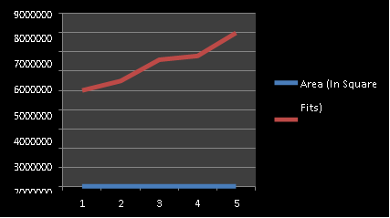
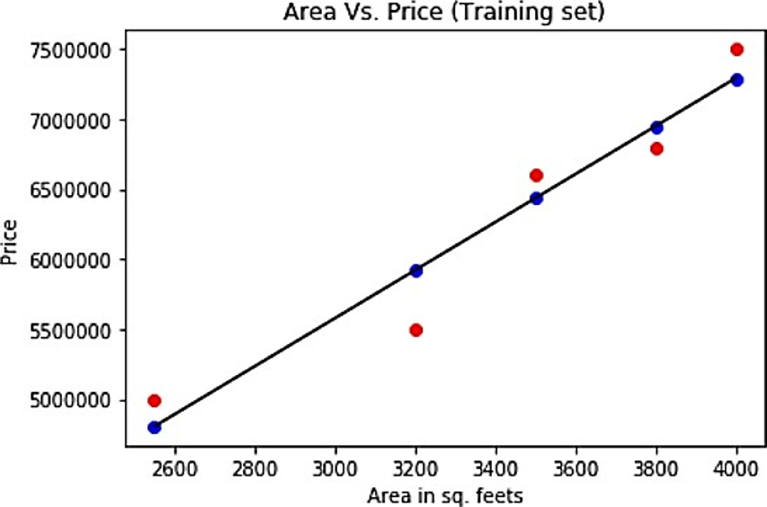
The program below fits a line to this table and predicts the price of a flat of 4,500 square feet. It is Part 1 of the full program shown in the next section. The complete code, including the imports the original page left out, is below.

Multiple Linear Regression

Multiple linear regression has two or more inputs. The equation grows to y = m1x1 + m2x2 + … + mnxn + c, where x1 to xn are the inputs and m1 to mn are their coefficients. Each coefficient shows the effect of that input while the others are held fixed.

For houses, the inputs could be area, number of bedrooms and age of the building, and the output is the price. The original page promised a table for this example but never showed it. In Part 2 below, I use a small table of 10 homes that I made up, with prices in lakh rupees.

Linear Regression in Python With scikit learn

This program has three parts. Part 1 is the simple example with five flats. Part 2 is the multiple example with three inputs. Part 3 uses the diabetes dataset that comes with scikit learn, with 442 patients, to show how to test a model properly on unseen data. All imports are included.

import numpy as np
import pandas as pd
from sklearn.datasets import load_diabetes
from sklearn.dummy import DummyRegressor
from sklearn.linear_model import LinearRegression
from sklearn.metrics import mean_absolute_error, mean_squared_error, r2_score
from sklearn.model_selection import train_test_split

# Part 1: simple linear regression, one input
house = pd.DataFrame({
    "area": [2550, 3200, 3500, 3800, 4000],
    "price": [5000000, 5500000, 6600000, 6800000, 7500000],
})
X = house[["area"]]
y = house["price"]
model = LinearRegression().fit(X, y)
print("Slope (price per extra sq ft):", round(model.coef_[0], 1))
print("Intercept:", round(model.intercept_, 1))
print("R squared on these 5 rows:", round(model.score(X, y), 3))
print("Predicted price for 4500 sq ft:", round(model.predict(pd.DataFrame({"area": [4500]}))[0]))

# Part 2: multiple linear regression, three inputs (made up data)
homes = pd.DataFrame({
    "area":     [1200, 1800, 1500, 2200, 2000, 2800, 2500, 3300, 3000, 3600],
    "bedrooms": [2, 3, 2, 3, 4, 4, 3, 5, 4, 5],
    "age":      [15, 5, 20, 10, 2, 12, 6, 8, 18, 3],
    "price":    [54, 84, 61, 102, 98, 123, 116, 149, 131, 166],
})
Xm = homes[["area", "bedrooms", "age"]]
multi = LinearRegression().fit(Xm, homes["price"])
for name, coef in zip(Xm.columns, multi.coef_):
    print(name, "coefficient:", round(float(coef), 3))
print("Intercept:", round(float(multi.intercept_), 2))
print("R squared on these 10 rows:", round(multi.score(Xm, homes["price"]), 3))
new = pd.DataFrame({"area": [2400], "bedrooms": [3], "age": [6]})
print("Predicted price (lakh) for 2400 sq ft, 3 bedrooms, 6 years old:", round(multi.predict(new)[0], 1))

# Part 3: judging a model properly on unseen data
data = load_diabetes()
X_train, X_test, y_train, y_test = train_test_split(
    data.data, data.target, test_size=0.3, random_state=0
)
lin = LinearRegression().fit(X_train, y_train)
pred = lin.predict(X_test)
print("Train R squared:", round(lin.score(X_train, y_train), 3))
print("Test R squared:", round(r2_score(y_test, pred), 3))
print("Test MAE:", round(mean_absolute_error(y_test, pred), 1))
print("Test RMSE:", round(float(np.sqrt(mean_squared_error(y_test, pred))), 1))
flat = DummyRegressor(strategy="mean").fit(X_train, y_train)
print("Flat average line, test R squared:", round(flat.score(X_test, y_test), 3) + 0.0)

Slope (price per extra sq ft): 1715.2
Intercept: 431269.3
R squared on these 5 rows: 0.925
Predicted price for 4500 sq ft: 8149536
area coefficient: 0.044
bedrooms coefficient: 0.123
age coefficient: -0.684
Intercept: 10.6
R squared on these 10 rows: 0.998
Predicted price (lakh) for 2400 sq ft, 3 bedrooms, 6 years old: 111.4
Train R squared: 0.554
Test R squared: 0.393
Test MAE: 44.6
Test RMSE: 55.7
Flat average line, test R squared: 0.0

Part 1: Simple Linear Regression Results

Slope (price per extra sq ft): 1715.2
Intercept: 431269.3
R squared on these 5 rows: 0.925
Predicted price for 4500 sq ft: 8149536

• The slope is 1,715.Each extra square foot adds about Rs 1,715 to the price.
• The prediction for 4,500 square feet is about Rs 81.5 lakh.That is 1,715.2 times 4,500 plus 431,269.
• Be careful with this prediction.The data only goes up to 4,000 square feet, and 4,500 is outside it. Predicting beyond your data is called extrapolation, and it is risky because the straight line may not continue.
• R squared of 0.925 is on only 5 rows,and the same rows were used to fit the line. With so few points, treat it as a demonstration, not a result.

Part 2: Multiple Linear Regression Results

area coefficient: 0.044
bedrooms coefficient: 0.123
age coefficient: -0.684
Intercept: 10.6
R squared on these 10 rows: 0.998
Predicted price (lakh) for 2400 sq ft, 3 bedrooms, 6 years old: 111.4

• Area:each extra square foot adds about 0.044 lakh, or Rs 4,400, holding the others fixed.
• Age:each extra year of age lowers the price by about 0.68 lakh. The negative sign shows a negative relationship.
• Bedrooms:the coefficient is small at 0.123, because bigger homes already have more bedrooms, and area captures most of the effect. When inputs overlap like this, the coefficients become unstable on small data.
• R squared of 0.998 is very high because I made the data up with little noise.Real data is never this clean.

In the original page’s code, the target was swapped and the model was misspelt. Here the target is price, and the prediction is made for a home of 2,400 square feet with 3 bedrooms and 6 years of age.

Part 3: Testing on Data the Model Has Not Seen

Train R squared: 0.554
Test R squared: 0.393
Test MAE: 44.6
Test RMSE: 55.7
Flat average line, test R squared: 0.0

• Test R squared is lower than train.The model scores 0.554 on the data it learned from and 0.393 on new data. The original page only ever checked the training data, so it would have shown the higher number.
• R squared is not accuracy.It is the share of the variation in the outcome that the model explains. A score of 0.393 means it explains about 39 percent.
• MAE and RMSE are in the units of the target.On average, predictions are off by about 44.6, and RMSE, which punishes big misses more, is 55.7.
• A flat average line scores 0.0.That is the baseline. The model beats it, so it has learned something, though not a great deal on this data.
• R squared can go below zero.A model that does worse than the flat average line scores a negative number. The original page says it is between 0 and 1, which is not always true.

Key Measures of a Regression Model

Assumptions of Linear Regression

1. A straight line relationship between each input and the outcome.
2. Independent errors. One row’s error should not predict another’s.
3. Constant spread of errors. The gaps should be about the same size across all predictions.
4. Errors roughly normal,which matters mainly when you want confidence intervals.
5. Little overlap between inputs. Strongly related inputs make coefficients unstable, as the bedrooms example shows.

Inputs must be numbers. If you have categories such as city or colour, encode them first.

Advantages and Disadvantages of Regression analysis

Advantages

• Simple, fast and easy to explain to anyone.
• Coefficients show the effect of each input.
• A strong baseline for any numeric prediction.
• Works with small data.

Disadvantages

• Assumes a straight line, so it misses curved patterns.
• Sensitive to outliers, because squared errors punish extreme points.
• Overlapping inputs make coefficients unstable.
• Predictions outside the range of the data can be unreliable.

Where Regression Analysis is Used?

• Real estate.Estimating property prices.
• Forecasting sales from price, season and promotions.
• Estimating risk and returns.
• Linking measurements such as weight or age to health outcomes.
• Predicting output or machine wear from operating conditions.
• Forecasting power and water demand.

Common Mistakes to Avoid

• Judging by training data only. Always check on held out data.
• Calling R squared accuracy. It measures fit, not accuracy.
• Predicting far outside the data. Like 4,500 square feet from data that ends at 4,000.
• Mixing up the target and the inputs. Check which column is y.
• Feeding in categories as text. Encode them first.
• Reading coefficients on overlapping inputs. They can swing wildly.
• Mistaking a link for a cause. Regression shows a relationship, not that one thing causes the other.

Regression analysis turns a table of numbers into a formula you can use and explain. Start with one input, then add more, and always test the result on data the model has not seen. Run the program above, replace my sample homes with your own data, and compare the model with a flat average line before you trust it. When the pattern bends, look at polynomial regression or a decision tree.