Logistic Regression in Machine Learning

A bank wants to know whether a loan applicant will default. A hospital wants to know whether a tumour is malignant. Your email app wants to know whether a message is spam. In each case the answer is not a number on a scale. It is a choice between categories, and the useful output is a probability, such as an 85 percent chance of default. Logistic regression is the classic tool for this job.

Despite its name, logistic regression is a classification algorithm. It takes the same weighted sum of inputs that linear regression uses, then passes it through a curve called the sigmoid function, which squeezes any number into a value between 0 and 1. That value is read as a probability. Because it is fast, easy to explain and gives probabilities, it is often the first model a team tries, and the baseline everything else must beat.

In this tutorial, we explain what logistic regression is, why a straight line fails for classification, and how the sigmoid function fixes it. We cover the types of logistic regression, the real assumptions behind it, and then run a complete Python example with output from an actual run, including accuracy, a comparison against a simple baseline, and the effect of changing the decision threshold. We end with strengths, limits, common mistakes and a short FAQ.

What is Logistic Regression?

Logistic regression is a supervised learning algorithm that predicts the probability that an input belongs to a category. The inputs, called independent variables or features, can be numbers or categories. The output, called the dependent variable, is a category, such as yes or no.

Some everyday examples:

• Will it rain tomorrow, yes or no?
• Is this transaction fraud, yes or no?
• Will this customer buy, yes or no?

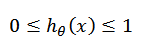
The model first calculates a score from the inputs. It then passes that score through the sigmoid function, so the final output is a probability. A common rule is that a probability of 0.5 or more means the positive class, and anything lower means the negative class.

Types of Logistic Regression

Binary Logistic Regression

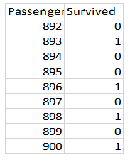
The outcome has exactly two values, such as 0 and 1, or true and false. A classic example is whether a Titanic passenger survived or not, based on age, ticket class and Gender.

Multinomial Logistic Regression

The outcome has more than two categories that have no natural order. For example, the weather could be sunny, cloudy or overcast. The model gives one probability for each category, and the probabilities add up to 1. The original page calls this multi linear logistic regression, but the correct name is multinomial.

Here is a small illustrative table of the kind of data involved. The values are made up to show the layout.

Ordinal Logistic Regression

A third type applies when the categories have a natural order, such as low, medium and high. Only this type depends on order.

Why Not Just Use Linear Regression?

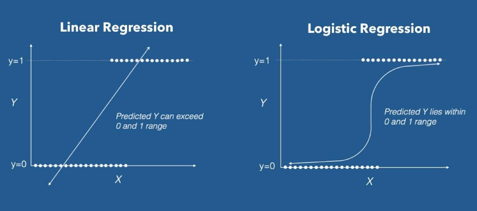
Linear regression draws a straight line, and a straight line has no limits. It can predict 1.7 or minus 0.4, which make no sense as probabilities. A few extreme points can also tilt the line and shift every prediction. We need a curve that stays between 0 and 1.

What is the Sigmoid Function?

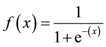
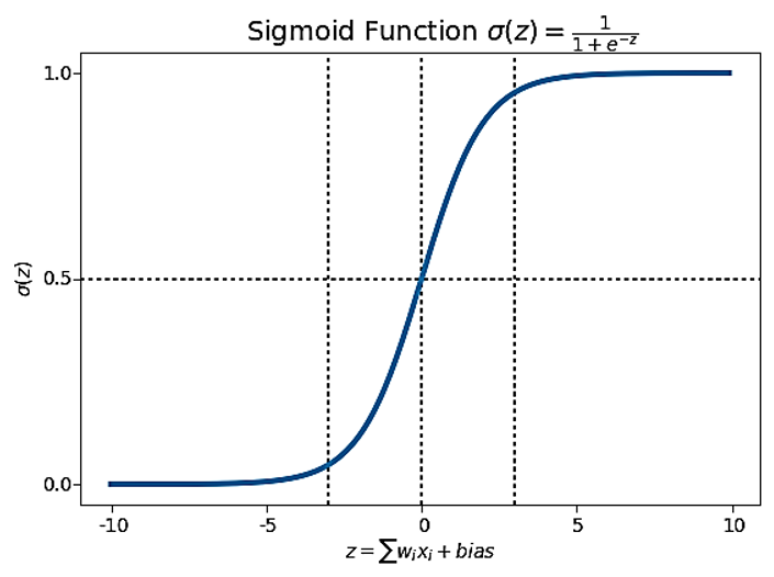
The sigmoid function takes any real number and maps it to a value between 0 and 1. It is shaped like a stretched letter S. Large positive numbers go close to 1, large negative numbers go close to 0, and zero maps exactly to 0.5. The formula is 1 divided by 1 plus e raised to the power of minus z, where z is the weighted sum of the inputs.

I checked these values by running them. Notice how a change from 0 to 2 moves the probability a lot, while a change from 2 to 4 moves it very little. The curve flattens at the ends.

Note that the sigmoid limits the model output, which is the prediction. It does not limit the cost function, as the original page says.

Odds and Log Odds, in Plain Words

Probability tells you how likely something is. Odds compare the chance of it happening with the chance of it not happening. If the probability is 0.75, the odds are 0.75 to 0.25, which is 3 to 1. The log odds are the natural logarithm of the odds.

Here is the key idea. Logistic regression assumes the log odds change in a straight line with the inputs. The sigmoid then converts the log odds back into a probability. That is what makes the model easy to interpret: each coefficient tells you how much the log odds change when that input rises by one unit.

Assumptions of Logistic Regression

These are the real assumptions, and a few things that people often confuse with them.

1. The outcome is categorical.Binary for the basic model, more categories for multinomial or ordinal. Order matters only for ordinal.
2. Observations are independent.Each row should not depend on another, so repeated measures of the same person break this.
3. Little multicollinearity.The inputs should not be strongly correlated with each other. They do not need to be fully independent.
4. A straight line relationship with the log odds.Between each numeric input and the log odds of the outcome, not the outcome itself.
5. No extreme outliers that dominate.A few very unusual points can pull the fit.

Two items from the original list are not assumptions. A sample size rule such as 50 observations per input is a rule of thumb. Handling missing values is a data preparation step, done before you fit the model.

Logistic Regression in Python With scikit learn

This program uses the breast cancer dataset that comes with scikit learn, with 569 patients and 30 measurements each. The label is malignant or benign. The program checks the sigmoid values, trains a model, compares it with a baseline, shows a confusion matrix, tests the effect of the threshold and ends with a three class example on the Iris dataset.

import numpy as np
from sklearn.datasets import load_breast_cancer, load_iris
from sklearn.linear_model import LogisticRegression
from sklearn.metrics import confusion_matrix, classification_report
from sklearn.model_selection import train_test_split
from sklearn.pipeline import make_pipeline
from sklearn.preprocessing import StandardScaler

# The sigmoid function
def sigmoid(z):
    return 1 / (1 + np.exp(-z))

for z in [-4, -2, 0, 2, 4]:
    print("z =", z, "probability =", round(float(sigmoid(z)), 3))

# Binary logistic regression
data = load_breast_cancer()
X, y = data.data, data.target
X_train, X_test, y_train, y_test = train_test_split(
    X, y, test_size=0.3, random_state=0, stratify=y
)
model = make_pipeline(StandardScaler(), LogisticRegression(max_iter=1000))
model.fit(X_train, y_train)
print("Test accuracy:", round(model.score(X_test, y_test), 3))
print("Baseline (always guess the common class):", round(max(y_test.mean(), 1 - y_test.mean()), 3))
print(confusion_matrix(y_test, model.predict(X_test)))
print(classification_report(y_test, model.predict(X_test), target_names=data.target_names))

# Probabilities and the threshold
proba = model.predict_proba(X_test)[:, 1]
for t in [0.5, 0.8]:
    pred = (proba >= t).astype(int)
    tn, fp, fn, tp = confusion_matrix(y_test, pred).ravel()
    print("threshold", t, "false positives", fp, "false negatives", fn)

# Multiclass (three outcomes) on Iris
Xi, yi = load_iris(return_X_y=True)
Xi_train, Xi_test, yi_train, yi_test = train_test_split(
    Xi, yi, test_size=0.3, random_state=0, stratify=yi
)
multi = make_pipeline(StandardScaler(), LogisticRegression(max_iter=1000)).fit(Xi_train, yi_train)
print("Iris three class accuracy:", round(multi.score(Xi_test, yi_test), 3))
print("Probabilities for one flower:", multi.predict_proba(Xi_test[:1]).round(3))

z = -4 probability = 0.018
z = -2 probability = 0.119
z = 0 probability = 0.5
z = 2 probability = 0.881
z = 4 probability = 0.982
Test accuracy: 0.959
Baseline (always guess the common class): 0.626
[[ 61   3]
 [  4 103]]
              precision    recall  f1-score   support

   malignant       0.94      0.95      0.95        64
      benign       0.97      0.96      0.97       107

    accuracy                           0.96       171
   macro avg       0.96      0.96      0.96       171
weighted avg       0.96      0.96      0.96       171

threshold 0.5 false positives 3 false negatives 4
threshold 0.8 false positives 2 false negatives 7
Iris three class accuracy: 0.978
Probabilities for one flower: [[0.    0.036 0.964]]

Part 1: Accuracy and the Baseline

When I ran the program, it printed:

Test accuracy: 0.959
Baseline (always guess the common class): 0.626

The test set has 171 patients. A lazy model that always guesses benign would be right 62.6 percent of the time, so any accuracy must be judged against that number. The original page reports 78.35 percent with no baseline and no dataset name, so a reader cannot tell whether that is good.

Part 2: The Confusion Matrix

[[ 61   3]
 [  4 103]]

Out of 64 malignant cases, 61 were found and 3 were called benign. Out of 107 benign cases, 4 were flagged as malignant. The precision and recall for each class were between 0.94 and 0.97.

Part 3: Moving the Threshold

The 0.5 cut off is a default, not a law. Here the model’s probability is for the benign class, and I tried raising the bar to 0.8:

threshold 0.5 false positives 3 false negatives 4
threshold 0.8 false positives 2 false negatives 7

Here, a false positive means a malignant case called benign, which is the costly mistake. Raising the threshold to 0.8 cut those from 3 to 2, but false negatives, which are benign cases flagged as malignant, rose from 4 to 7. You always trade one kind of error for the other. Choose the threshold based on which mistake costs more in your business, not on the default.

Part 4: Three Outcomes

Iris three class accuracy: 0.978
Probabilities for one flower: [[0.    0.036 0.964]]

With three flower species, the same model gives one probability for each, and they add up to 1. For the flower shown, the model is 96.4 percent sure of the third species. The test set has 45 flowers, so 0.978 means 44 correct.

Key Settings in LogisticRegression

Strengths and Limitations of Logistic Regression

Strengths

• Simple, fast and easy to explain.
• Gives probabilities, not only labels.
• Coefficients show how each input affects the outcome.
• Works well as a first model and a baseline.
• Needs little tuning and trains quickly on large data.

Limitations

• Assumes a straight line relationship with the log odds, so it can miss curved patterns.
• Can struggle when classes cannot be separated by a flat boundary.
• Sensitive to correlated inputs and to scale, if you use regularization.
• Needs a threshold choice for imbalanced classes.

Where Logistic Regression is Used?

• Credit scoring and loan default.
• Disease risk from patient measurements.
• Predicting whether a lead will convert.
• Spam filtering.
• Predicting whether equipment will fail.

Common Mistakes to Avoid

• Reporting accuracy without a baseline. Always compare with a lazy model.
• Ignoring the threshold. The default of 0.5 may not suit your costs.
• Forgetting to scale. It helps convergence and regularization.
• Using it on curved patterns without extra features. Add terms or choose another model.
• Leaving highly correlated inputs. The coefficients become unstable.
• Calling it regression for numbers. It predicts categories.

Logistic regression is a small idea that goes a long way. A weighted sum, a sigmoid curve and a threshold give you a model that is fast, explainable and surprisingly hard to beat. Run the program on your own data, compare it with a baseline, and choose your threshold with your costs in mind. If the pattern is curved, try a random forest next.