Outliers in Machine Learning: How to Detect and Handle Them

An HR manager is reviewing the salaries in a small company. Nineteen people earn between 30,000 and 60,000 rupees a month, and one earns 12 lakh. If the manager reports the average salary, the number will describe nobody. One person has pulled it far above what everyone else earns. That single value is an outlier, and it can mislead anything that depends on the average, including a machine learning model.

An outlier is a data point that sits far from the rest of the data. Some are mistakes, such as a typing error that turns 45 into 450. Others are completely real and extremely important, such as a fraudulent transaction or a failing machine. Treating them all the same way is the most common error beginners make, and it is the one that costs the most.

In this tutorial, we explain what outliers are, where they come from and how they affect a model. We then detect them in four ways: with a scatter plot, a box plot, the z score and the interquartile range. A tested Python program shows the numbers on real data, including a result that will surprise you: removing outliers can throw away the very cases you care about. We end with how to decide whether to keep, fix or remove an outlier, common mistakes and a short FAQ.

What is an Outlier?

An outlier is an observation that is very different from the rest of the values in a dataset. It may be unusually high, unusually low, or just an odd combination of values.

Where Do Outliers Come From?

• Typing mistakes, a faulty sensor, a wrong unit such as grams entered as kilograms.
• Natural variation.Some people really are very tall, and some customers really do spend 50 times the average.
• Rare events.Fraud, equipment failure, an unusual disease. These are often the point of the exercise.
• Mixed groups.Data from two different populations that were accidentally combined.

Effects of Outliers on Data and Models

Outliers distort measures that use every value. The mean and the standard deviation are the two most affected. In the breast cancer data used below, the mean tumour area is 654.9, but the median is 551.1. The gap of about 100 is caused by a long tail of very large tumours. The mean has been pulled up, and the median has not.

Models are affected too. Linear regression is sensitive, because it minimises squared errors, and one extreme point has an outsized pull. In the program below, I generated 20 points around a line with a slope of about 3. With all points normal, the fitted slope was 2.94. After changing just the last point to a bad value, the slope dropped to 2.06. One point out of 20 changed the answer by almost a third.

Types of Outliers

• Univariate outliersare unusual in a single variable. A salary of 12 lakh in a column of salaries is one.
• Multivariate outliersare unusual only when you consider several variables together. A person who is 150 cm tall is normal, and a weight of 100 kg is normal, but 150 cm and 100 kg together may be rare. Each value looks fine alone.

Multivariate outliers are harder to spot, because no single column looks wrong. They need methods that look at several columns at once.

How to Identify Outliers?

There are two families of methods. Visual methods let you see the data. Statistical methods put a number on how unusual a point is. Use both, since a chart often explains what a number cannot.

Finding Outliers With Visual Tools

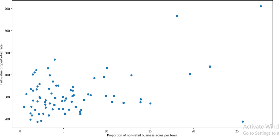
Using a Scatter Plot

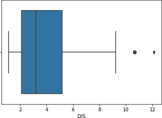
A scatter plot puts one variable on each axis. Points that sit far from the main cloud are suspects. It is the quickest way to spot an outlier that involves two variables. The code below draws a scatter plot, then a box plot, using the breast cancer dataset that comes with scikit learn, which has 569 patients and 30 measurements each.

import matplotlib.pyplot as plt
from sklearn.datasets import load_breast_cancer

df = load_breast_cancer(as_frame=True).frame

# Scatter plot: two variables at once
plt.scatter(df["mean area"], df["mean smoothness"], alpha=0.5)
plt.xlabel("Mean area")
plt.ylabel("Mean smoothness")
plt.title("Mean area against mean smoothness")
plt.show()

# Box plot: one variable
plt.boxplot(df["mean area"])
plt.ylabel("Mean area")
plt.title("Box plot of mean area")
plt.show()

Using a Box Plot

A box plot shows one variable. The box covers the middle half of the values, from the first to the third quartile. The line inside is the median. The whiskers reach to the furthest values within 1.5 times the box length, and any dot beyond a whisker is drawn as a possible outlier.

Finding Outliers With Mathematical Methods

The program in the next block runs the numbers for all the methods below. Here is each method in words first.

Using the Z Score

The z score tells you how many standard deviations a value is from the mean. You subtract the mean from the value and divide by the standard deviation. A common rule flags any point with a z score above 3 or below minus 3.

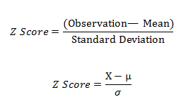
Two cautions apply. The rule of 3 works best when the data is roughly bell shaped. And the mean and standard deviation are themselves pulled by outliers, so extreme points can hide each other. A z score only rescales data. It does not tell you what distribution the data follows, which the original page wrongly suggests.

Using the Interquartile Range

The interquartile range, or IQR, is the distance between the third quartile, Q3, and the first quartile, Q1. A point is flagged as an outlier if it is more than 1.5 times the IQR below Q1, or more than 1.5 times the IQR above Q3. Because it uses quartiles, it does not depend on the mean, and it works for skewed data. The IQR is calculated for each column, not each row.

Using an Isolation Forest

An isolation forest is built to find multivariate outliers. It builds many random trees. Points that are unusual get separated from the rest in very few splits, so they are easy to isolate. It looks at all columns together, which is why it can catch odd combinations that no single column reveals.

Outlier Detection in Python

This program runs all four methods on the mean tumour area, then on all 30 columns, shows what removal costs, and tests the effect on a regression line.

import numpy as np
import pandas as pd
from scipy import stats
from sklearn.datasets import load_breast_cancer
from sklearn.ensemble import IsolationForest
from sklearn.linear_model import HuberRegressor, LinearRegression

data = load_breast_cancer(as_frame=True)
df = data.frame.drop(columns="target")
col = df["mean area"]

# Part 1: one column, two methods
print("Rows:", len(col))
print("Mean:", round(col.mean(), 1), "Median:", round(col.median(), 1), "Max:", col.max())

z = np.abs(stats.zscore(col))
print("Z score method, |z| > 3:", int((z > 3).sum()))

Q1, Q3 = col.quantile(0.25), col.quantile(0.75)
IQR = Q3 - Q1
lower, upper = Q1 - 1.5 * IQR, Q3 + 1.5 * IQR
print("IQR:", round(IQR, 1), "fences:", round(lower, 1), "to", round(upper, 1))
print("IQR method:", int(((col < lower) | (col > upper)).sum()))

# Part 2: all 30 columns, and what removal costs
z_all = np.abs(stats.zscore(df))
print("Rows with any |z| > 3:", int((z_all > 3).any(axis=1).sum()), "of", len(df))
Q1a, Q3a = df.quantile(0.25), df.quantile(0.75)
IQRa = Q3a - Q1a
mask = ((df < Q1a - 1.5 * IQRa) | (df > Q3a + 1.5 * IQRa)).any(axis=1)
print("Rows with any IQR outlier:", int(mask.sum()), "of", len(df))
print("Share of malignant cases among removed rows:", round(float((data.target[mask] == 0).mean()), 3))
print("Share of malignant cases overall:", round(float((data.target == 0).mean()), 3))

# Part 3: one bad point against a regression line
x = np.arange(1, 21).reshape(-1, 1)
y = 3 * x.ravel() + 5 + np.random.default_rng(0).normal(0, 2, 20)
y_bad = y.copy()
y_bad[-1] = 5
print("Slope without the bad point:", round(LinearRegression().fit(x, y).coef_[0], 2))
print("Slope with the bad point:", round(LinearRegression().fit(x, y_bad).coef_[0], 2))
print("Huber slope with the bad point:", round(HuberRegressor().fit(x, y_bad).coef_[0], 2))

# Part 4: outliers across several columns at once
forest = IsolationForest(contamination=0.05, random_state=0).fit(df)
print("Isolation forest flags:", int((forest.predict(df) == -1).sum()), "rows")

Rows: 569
Mean: 654.9 Median: 551.1 Max: 2501.0
Z score method, |z| > 3: 8
IQR: 362.4 fences: -123.3 to 1326.3
IQR method: 25
Rows with any |z| > 3: 74 of 569
Rows with any IQR outlier: 171 of 569
Share of malignant cases among removed rows: 0.667
Share of malignant cases overall: 0.373
Slope without the bad point: 2.94
Slope with the bad point: 2.06
Huber slope with the bad point: 2.87
Isolation forest flags: 29 rows

print(“Isolation forest flags:”, int((forest.predict(df) == -1).sum()), “rows”)

Part 1: One Column, Two Methods

Rows: 569
Mean: 654.9 Median: 551.1 Max: 2501.0
Z score method, |z| > 3: 8
IQR: 362.4 fences: -123.3 to 1326.3
IQR method: 25

• The two methods disagree.The z score flagged 8 values, and the IQR rule flagged 25. Neither is wrong. They use different definitions of unusual.
• The reason is skew.Tumour area has a long tail to the right, so it is not bell shaped, and the z score rule is less suited to it.
• The lower fence is negative at minus 123.3.An area cannot be negative, so there are no low outliers here. That is a good reminder to check fences against what is physically possible.

Part 2: What Removal Really Costs

Rows with any |z| > 3: 74 of 569
Rows with any IQR outlier: 171 of 569
Share of malignant cases among removed rows: 0.667
Share of malignant cases overall: 0.373

This is the most important result. Applied to all 30 columns, the z score rule would drop 74 rows, and the IQR rule would drop 171, which is 30 percent of the whole dataset. Worse, 66.7 percent of the rows the IQR rule would remove are malignant cases, while malignant cases are only 37.3 percent of the data. The unusual rows are unusual because they are the serious cases. A cleaning step that removes them would make a cancer model blind to cancer.

The original page says outliers should be excluded. This result shows why that rule is dangerous.

Part 3: One Bad Point and a Regression Line

Slope without the bad point: 2.94
Slope with the bad point: 2.06
Huber slope with the bad point: 2.87

One bad point in 20 pulled the ordinary linear regression slope from 2.94 to 2.06. A Huber regressor, which is built to give extreme points less weight, got 2.87 on the same bad data, close to the truth. When you cannot decide whether to remove a point, a method that is resistant to outliers is often better than deleting it.

Part 4: Isolation Forest

Isolation forest flags: 29 rows

With the contamination setting at 0.05, the isolation forest flagged 29 of 569 rows, which is about 5 percent. That number is set by you, not discovered by the model, so treat it as a shortlist to inspect, not a verdict.

What to Do With an Outlier

Detection is only half the job. Before you change anything, ask why the point is unusual.

Options besides removal include capping extreme values at a limit, which is called winsorizing, applying a log transformation to a long tail, and using models that are naturally resistant to outliers, such as tree based models or the Huber regressor.

Common Mistakes to Avoid

• Deleting outliers automatically. Check the cause first. Our example would have removed 171 rows, mostly the serious cases.
• Using the z score on skewed data. Use IQR, or transform the data first.
• Removing a row because one column looks odd. Dropping a whole row for an outlier in any of 30 columns throws away a lot of good data.
• Checking one column at a time only. Multivariate outliers will be missed.
• Cleaning before splitting the data. Decide on the rules using training data, then apply the same rules to test data.
• Forgetting what is physically possible. A negative fence for a quantity that cannot be negative tells you the method does not fit.
• Not recording what you removed. Keep a list so the cleaning can be explained.

Outliers are not just dirty data to be scrubbed away. Sometimes they are mistakes, and sometimes they are the story. Learn the four ways to spot them, check each against the physical reality of your data, and compare your results with and without them before you delete anything. Run the program above on your own dataset, and see how many rows each rule would remove.