Boosting Techniques in Machine Learning
Boosting Techniques in Machine Learning
If you ask experienced data scientists which algorithm family wins most competitions on tables of data, many of them give the same answer: boosting. Methods such as XGBoost, LightGBM and CatBoost sit behind a large share of fraud detection, credit scoring, click prediction and sales forecasting systems. They are rarely the most glamorous models, but they are often the most accurate ones on structured data.
The idea behind boosting is simple and rather human. A single weak model, one that is only a little better than guessing, is not much use alone. But if you train a second model that concentrates on the mistakes of the first, and a third that concentrates on the mistakes that remain, and then combine them all, the group can become very accurate. Boosting is a way of turning many weak learners into one strong learner.
This guide explains how boosting works, how it differs from bagging, and then covers the five best known techniques: AdaBoost, Gradient Boosting, XGBoost, LightGBM and CatBoost. You will see a small worked example you can follow by hand, and a complete Python program that compares all five on the same data. We finish with tuning advice, applications, common mistakes and a short FAQ.
What is Boosting?
Boosting is an ensemble method, which means it combines several models into one. What makes it special is that the models are built in sequence. Each new model is trained to fix the errors left by the models before it. When it is time to predict, the models vote or add up their outputs, usually giving stronger models more say.
The base models are usually very small decision trees, sometimes only a single split, called a stump. A stump alone is a poor predictor, which is exactly the point. Boosting steadily reduces bias, the error that comes from a model being too simple to capture the pattern.
Bagging Versus Boosting
| Point | Bagging | Boosting |
|---|---|---|
| Main goal | Reduce variance | Reduce bias, step by step |
| How models are built | Independently, in parallel | One after another, each fixing the last |
| Best base models | Strong, complex ones such as full trees | Weak, simple ones such as shallow trees |
| Data for each model | Random samples of the data | The same data, re weighted or fitted to the errors |
| Famous example | Random forest | AdaBoost, XGBoost |
| Risk | Little | Can overfit if run too long on noisy data |
The Five Boosting Techniques at a Glance
| Technique | Core idea | Notable strength |
|---|---|---|
| AdaBoost | Re weights the training examples so later models focus on the ones that were wrong | Simple, the original boosting method |
| Gradient Boosting | Each new tree is fitted to the errors, called residuals, of the current model | Flexible, works with many loss functions |
| XGBoost | An optimised gradient boosting with built in regularisation | Strong accuracy, handles missing values |
| LightGBM | Gradient boosting that grows trees leaf by leaf and bins the data into histograms | Very fast on large data |
| CatBoost | Gradient boosting designed to handle categorical columns directly | Needs little preprocessing for categories |
1. AdaBoost
AdaBoost, short for adaptive boosting, was introduced in 1995 by Freund and Schapire. It starts by giving every training example the same weight. After each weak model is trained, the examples it got wrong are given more weight, and the ones it got right are given less. The next model is therefore pushed to concentrate on the hard cases.
Here is the process in steps:
- Give every example an equal weight.
- Train a weak model, usually a stump, using the weights.
- Measure its weighted error, the share of weight on examples it got wrong.
- Give the model a say, called alpha, that grows as its error shrinks.
- Increase the weights of the examples it got wrong, decrease the weights of the others, and rescale so the weights add up to one.
- Repeat for the chosen number of rounds, then combine all the models using their say.
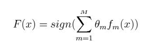
The say of each model and the final prediction for a two class problem are:
alpha_m = 0.5 * ln( (1 – error_m) / error_m )
F(x) = sign( alpha_1 * f_1(x) + alpha_2 * f_2(x) + … + alpha_M * f_M(x) )
Here f_m is the m th weak model and the output of each is plus one or minus one. The sign of the weighted sum is the final class.
:
To see the effect, here is a short experiment on the breast cancer dataset. A single stump is compared with AdaBoost made of stumps.
from sklearn.datasets import load_breast_cancer
from sklearn.model_selection import train_test_split
from sklearn.tree import DecisionTreeClassifier
from sklearn.ensemble import AdaBoostClassifier
X, y = load_breast_cancer(return_X_y=True)
X_train, X_test, y_train, y_test = train_test_split(X, y, test_size=0.25, random_state=0, stratify=y)
stump = DecisionTreeClassifier(max_depth=1).fit(X_train, y_train)
print(“One stump:”, round(stump.score(X_test, y_test), 3))
for n in [10, 50, 100]:
ada = AdaBoostClassifier(n_estimators=n, random_state=0).fit(X_train, y_train)
print(n, “rounds:”, round(ada.score(X_test, y_test), 3))
A single stump scored 0.888 on the test set. AdaBoost with only 10 rounds reached 0.944. Notice that 100 rounds did not do better here, scoring 0.930. More rounds do not always help, which is why you should check performance on data the model has not seen.
One stump: 0.888
10 rounds: 0.944
50 rounds: 0.944
100 rounds: 0.93
2. Gradient Boosting
Gradient boosting takes a different route to the same destination. Instead of re weighting examples, each new tree is trained to predict the residuals, the gap between the current prediction and the true value. Adding that correction moves the model closer to the truth. A small multiplier called the learning rate controls how big each correction is.
A tiny example makes this concrete. Suppose we want to predict weight in kilograms for five people, ordered by height, and the true values are 50, 60, 70, 80 and 90.
- Start with the average.Predict 70 for everyone. The residuals are minus 20, minus 10, 0, 10 and 20.
- Fit a small tree to the residuals.A single split on height puts the two shortest people in one group, with an average residual of minus 15, and the three taller people in the other, with an average residual of plus 10.
- Add a fraction of the correction.With a learning rate of 0.5, the first two people are now predicted at 62.5 and the other three at 75.
- Check the improvement.The total squared error falls from 1,000 to 437.5.
The next tree is then fitted to the new residuals, and the process repeats. After enough rounds the predictions are close to the truth.
For large datasets, scikit learn recommends HistGradientBoostingClassifier, which is far faster than the classic GradientBoostingClassifier and handles missing values. For small datasets, the classic version is fine.
3. XGBoost
XGBoost, short for extreme gradient boosting, is a carefully engineered version of gradient boosting. Its key additions are regularisation, which penalises overly complex trees so they overfit less, built in handling of missing values, and an efficient implementation that uses all your processor cores. It is often much faster than older gradient boosting code, though how much depends on your data.
4. LightGBM
LightGBM, from Microsoft, makes boosting fast on big data. It groups feature values into histogram bins, and it grows each tree leaf wise, always splitting the leaf that reduces the error the most, instead of growing level by level. That gets accuracy quickly, but it can overfit on small datasets. If your data is small, limit the tree size with the num_leaves, max_depth and min_child_samples settings.
5. CatBoost
CatBoost, from Yandex, is built for data that has many categorical columns, such as city, product type or customer segment. It can take those columns directly, with no need to turn them into numbers by hand, and it uses a technique called ordered boosting to reduce a problem known as target leakage. It often gives good results with little tuning.
Comparing All Five on the Same Data
The page this guide replaces compared methods using different datasets, which makes the scores meaningless. Here is a fair comparison. Every model sees the same training and test split of the breast cancer dataset, and all use 100 trees and a learning rate of 0.1 where the setting applies. First install the libraries:
pip install scikit-learn xgboost lightgbm catboost
from sklearn.datasets import load_breast_cancer
from sklearn.model_selection import train_test_split
from sklearn.metrics import accuracy_score
from sklearn.ensemble import AdaBoostClassifier, GradientBoostingClassifier
from xgboost import XGBClassifier
from lightgbm import LGBMClassifier
from catboost import CatBoostClassifier
X, y = load_breast_cancer(return_X_y=True)
X_train, X_test, y_train, y_test = train_test_split(
X, y, test_size=0.25, random_state=0, stratify=y
)
models = {
“AdaBoost”: AdaBoostClassifier(n_estimators=100, random_state=0),
“Gradient Boosting”: GradientBoostingClassifier(n_estimators=100, learning_rate=0.1, random_state=0),
“XGBoost”: XGBClassifier(n_estimators=100, learning_rate=0.1, random_state=0),
“LightGBM”: LGBMClassifier(n_estimators=100, learning_rate=0.1, random_state=0, verbose=-1),
“CatBoost”: CatBoostClassifier(iterations=100, learning_rate=0.1, random_seed=0, verbose=0),
}
for name, model in models.items():
model.fit(X_train, y_train)
accuracy = accuracy_score(y_test, model.predict(X_test))
print(f”{name}: {accuracy:.3f}”)
When I ran it, the output was:
AdaBoost: 0.930
Gradient Boosting: 0.958
XGBoost: 0.951
LightGBM: 0.944
CatBoost: 0.944
All five land within about three percentage points of each other. On a test set of 143 patients, a single patient changes the score by 0.7 points, so you should not declare a winner from this table. On real projects, use cross validation and compare on your own data. The practical lesson is that boosting methods are all strong, and the best one depends on your data.
Which Boosting Method Should You Use?
| Your situation | Try first |
|---|---|
| Learning the idea, small data | AdaBoost or classic Gradient Boosting |
| Tabular data with up to a few hundred thousand rows | XGBoost or HistGradientBoosting |
| Millions of rows, speed matters | LightGBM |
| Many categorical columns | CatBoost |
| You want a strong default with little tuning | CatBoost or HistGradientBoosting |
Tuning Boosting Models
- Learning rate and number of trees go together. Smaller learning rates need more trees to reach the same fit, and usually generalise better. Scikit learn suggests a learning rate of 0.1 or lower, with enough trees that early stopping decides when to halt.
- Use early stopping. Hold back some data and stop adding trees when the score on it stops improving.
- Keep trees small. Shallow trees are the point of boosting. Deep trees overfit faster.
- Subsample the rows. Training each tree on a fraction of the data, such as half, often improves accuracy when combined with a small learning rate.
- Use the penalty settings in XGBoost, LightGBM and CatBoost to keep trees simple.
Applications of Boosting
- Credit scoring and fraud detection. Boosted trees are common in banking.
- Click and conversion prediction. Ranking ads and recommendations.
- Demand and sales forecasting. Predicting numbers from tables of past data.
- Customer churn and employee attrition. Finding who is likely to leave.
- Search ranking. Many ranking systems use boosted trees.
- Healthcare risk models. Predicting outcomes from patient measurements.
Common Mistakes
- Comparing scores from different datasets. A fair comparison needs the same data and split.
- Running too many rounds. Boosting can overfit, especially on noisy data. Use early stopping.
- Ignoring the learning rate. It must be tuned together with the number of trees.
- Using LightGBM defaults on a tiny dataset. Leaf wise growth can overfit, so limit the tree size.
- Marking numeric columns as categorical. In CatBoost, only list true category columns.
- Trusting one lucky test split. Use cross validation.
Boosting turns many modest models into one very accurate one by letting each learn from the mistakes of the last. Start with the comparison program on your own data, use cross validation to pick between the methods, and keep the learning rate small and early stopping on.