Reinforcement Learning Tutorial for Beginners
Reinforcement Learning Tutorial for Beginners
Most people meet machine learning through examples with answers attached. You show a program thousands of photos labelled cat or dog, and it learns to tell them apart. But a lot of real problems do not come with labelled answers. Nobody can hand a robot a list of the right move at every moment, and nobody can tell a game playing program the best move in every position. What exists instead is an outcome: the robot reached the door, or the game was won.
Reinforcement learning is the branch of machine learning built for exactly this situation. A program called an agent tries actions in an environment, receives rewards or penalties, and gradually works out which behaviour earns the most reward over time. It is how programs have learned to play board games and video games at expert level, how robots learn to walk or grasp objects, and how some systems learn to manage resources such as energy or traffic.
This tutorial explains reinforcement learning from the ground up, with no maths background assumed. We begin with the idea itself and an everyday example, then compare it with supervised and unsupervised learning. After that come the key terms, the exploration versus exploitation dilemma, Markov decision processes and the shortest path problem. Finally we go beyond definitions: value functions, Q learning, a short Python program you can run, the main families of algorithms, real applications, challenges and a short FAQ.
What Is Reinforcement Learning?
Reinforcement learning is learning by trial and error, guided by rewards. The learner is not told which action is correct. It acts, sees what happens, and adjusts. Actions that lead to good outcomes become more likely, and actions that lead to bad outcomes become less likely.
The goal is not to win any single step. It is to collect the largest total reward over the whole task. That distinction matters. Sometimes the best move now costs something, such as giving up a piece in chess, because it leads to a better result later. Reinforcement learning is about learning that long term thinking.
Framing Reinforcement Learning: A Child Learning to Ride a Bicycle
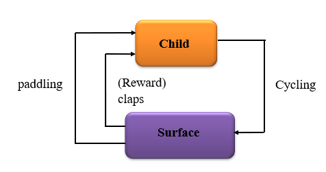
Think of a child learning to ride a bicycle. Nobody gives the child a rule book. The child pushes the pedals, wobbles, falls, tries again, and slowly finds the balance that keeps the bicycle upright.

In reinforcement learning terms, the child is the agent. The bicycle and the road are the environment. Pedalling, steering and braking are actions. How steady the bicycle feels at any moment is the state. Staying upright and moving forward feels good, which is a reward. Falling hurts, which is a penalty. Over many attempts, the child develops a policy, which is a habit for what to do in each situation.
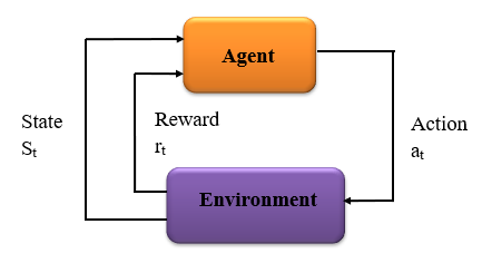
The same loop can be drawn for any task. The agent observes the state, picks an action, the environment responds with a new state and a reward, and the cycle repeats.
Reinforcement Learning Compared With Other Types of Machine Learning
| Point | Supervised learning | Unsupervised learning | Reinforcement learning |
|---|---|---|---|
| Learns from | Labelled examples | Unlabelled data | Rewards from interaction |
| Feedback | The correct answer for each example | None | A reward, often delayed |
| Goal | Predict labels or values | Find structure or groups | Maximise total reward |
| Data comes from | A fixed dataset | A fixed dataset | The agent’s own actions |
| Typical use | Spam detection, price prediction | Customer segments, anomaly detection | Games, robotics, control |
A key difference is that in reinforcement learning, the data depends on what the agent does. If it never tries a certain action, it never learns what that action would have earned.
Key Terms You Need to Know
| Term | Meaning |
|---|---|
| Agent | The learner and decision maker |
| Environment | Everything the agent interacts with |
| State | A description of the situation at a given moment |
| Action | A choice the agent can make |
| Reward | A number the environment returns after an action, positive for good outcomes and negative for bad ones |
| Policy | The agent’s strategy, a rule that says which action to take in each state |
| Value function | An estimate of how much total reward the agent can expect from a state, if it follows its policy |
| Discount factor | A number between 0 and 1 that makes future rewards count for less than immediate ones |
| Episode | One complete run from a starting state to an ending state |
The Exploration Versus Exploitation Dilemma
Imagine a row of slot machines, each paying out at a different, unknown rate. You have a limited number of coins. Do you keep playing the machine that has paid well so far, or do you try the others in case one is better?
- Exploitationmeans using what you already know to pick the best option found so far.
- Explorationmeans trying something less certain to learn more, even if it might pay less right now.
Too much exploitation and you may get stuck on an average machine while a much better one sits untried. Too much exploration and you waste coins on bad machines. Every reinforcement learning agent has to balance the two.
A simple and popular method is epsilon greedy. With a small probability, called epsilon, the agent picks a random action to explore. The rest of the time it picks the best known action. Many agents start with a high epsilon and lower it as they learn.
Markov Decision Processes (MDP)
To work on reinforcement learning problems mathematically, we describe them as a Markov decision process, usually shortened to MDP. An MDP has five parts: a set of states, a set of actions, rules for how actions change the state, rewards, and a discount factor.

The idea that gives the process its name is the Markov property. It says the future depends only on the current state and the action taken, not on the whole history of how you got there. A chess position is a good example. The best move depends on where the pieces are now, not on the order the moves were played.
A Worked Example: The Shortest Path Problem
Picture a map of connected nodes, where every road between two nodes has a cost, such as distance or travel time. The agent starts at one node and wants to reach a destination at the lowest total cost. In reinforcement learning terms, each node is a state, each road is an action, and each cost is a negative reward.
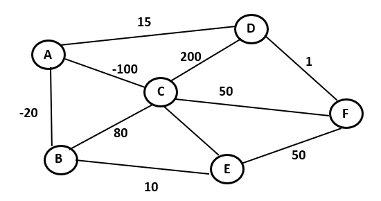
A simple approach is greedy: at every node, take the road with the lowest immediate cost. It is easy, but it can fail. A cheap first step can lead into a dead end or into expensive roads later, so the greedy path is not always the cheapest overall. An agent that explores different routes, and learns the total value of each choice, can discover better ones. That is the reason reinforcement learning tracks long term reward and not only the next step.
Value Functions and Q Learning
How does an agent actually learn? Most methods keep a score for every situation, estimating how good it is. There are two common versions:
- A state valuesays how good it is to be in a state.
- An action value, written Q, says how good it is to take a particular action in a particular state.
Q learning is one of the most famous algorithms. It keeps a table of Q values and updates one entry after every step using this rule:
Q(state, action) = Q(state, action) + alpha * (reward + gamma * best Q(next state) – Q(state, action))
In plain words: look at what actually happened, which is the reward you got plus the best value you expect from where you landed. Compare it with what you expected before. Then move your old estimate a small step towards the new evidence. Alpha is the learning rate, the size of that step. Gamma is the discount factor. Repeat this thousands of times and the table fills with good estimates.
A Short Q Learning Example in Python
Here is a complete program you can run. An agent walks along a corridor of six cells. It starts at the left end, and the goal is the right end. Every step costs one point, and reaching the goal gives ten. It uses epsilon greedy to balance exploration and exploitation.
import random
# A corridor of 6 cells. The agent starts at cell 0 and the goal is cell 5.
N_STATES = 6
ACTIONS = [0, 1] # 0 = move left, 1 = move right
alpha, gamma, epsilon = 0.1, 0.9, 0.2
Q = [[0.0, 0.0] for _ in range(N_STATES)]
def step(state, action):
next_state = max(0, state – 1) if action == 0 else min(N_STATES – 1, state + 1)
if next_state == N_STATES – 1:
return next_state, 10.0, True # reached the goal
return next_state, -1.0, False # every other move costs 1
random.seed(1)
for episode in range(500):
state, done = 0, False
while not done:
if random.random() < epsilon:
action = random.choice(ACTIONS) # explore
else:
action = max(ACTIONS, key=lambda a: Q[state][a]) # exploit
next_state, reward, done = step(state, action)
best_next = max(Q[next_state])
Q[state][action] += alpha * (reward + gamma * best_next – Q[state][action])
state = next_state
policy = [“right” if Q[s][1] >= Q[s][0] else “left” for s in range(N_STATES – 1)]
print(policy)
print([round(max(q), 1) for q in Q])
When I ran it, the output showed that the agent learned to move right in every cell, and the values rose steadily towards the goal:
[‘right’, ‘right’, ‘right’, ‘right’, ‘right’]
[3.1, 4.6, 6.2, 8.0, 10.0, 0.0]
Nobody told the agent that right was the correct direction. It found out from rewards alone. The last number is zero because the goal cell ends the episode.
Types of Reinforcement Learning Algorithms
| Family | Idea | Examples |
|---|---|---|
| Value based | Learn the value of actions and pick the best one | Q learning, Deep Q Networks |
| Policy based | Learn the policy directly | REINFORCE, policy gradient methods |
| Actor critic | Combine both, an actor picks actions and a critic scores them | A2C, PPO |
| Model free | Learn from experience without a model of the environment | Q learning, PPO |
| Model based | Learn or use a model of how the environment behaves, then plan | Dyna, planning methods |
When the number of states is too large for a table, as in video games or robotics, a neural network replaces the table. That combination is called deep reinforcement learning.
Practical Applications of Reinforcement Learning
- Programs have reached expert level in board games and video games by playing against themselves.
- Robots learn to walk, balance and pick up objects through practice, often in simulation first.
- Self driving and navigation. Decisions such as lane changes and route choice can be framed as reward problems.
- Resource management. Google DeepMind reported using reinforcement learning to reduce the energy used for cooling in data centres.
- Recommendations and personalisation. Systems can learn which suggestions keep users engaged over time.
- Trading strategies and portfolio decisions are studied as reinforcement learning problems, though real world results need careful testing.
- Training and education software. Adaptive systems can choose the next exercise to suit each learner.
Challenges of Reinforcement Learning
- Designing the reward. An agent maximises exactly what you reward. A badly designed reward gets exploited in surprising ways.
- Needs lots of experience. Many agents need millions of attempts, which is cheap in a simulator and costly in the real world.
- Delayed rewards. When the payoff comes much later, it is hard to know which earlier action deserves the credit.
- Exploring by trial and error is a problem when mistakes are expensive or dangerous.
- Unstable training. Results can vary a lot between runs, so careful testing is essential.
Common Mistakes Beginners Make
- Mixing up exploration and exploitation. Exploration tries new options. Exploitation uses the best known option.
- Calling greedy epsilon greedy. Epsilon greedy adds random exploration. Plain greedy does not.
- Rewarding the wrong thing. The agent will chase the reward you wrote, not the goal you meant.
- Forgetting the discount factor. Without it, the agent cannot weigh near rewards against distant ones.
- Starting with a hard problem. Begin with a tiny environment like the corridor above, and scale up.
Reinforcement learning is a simple idea with deep consequences: act, observe the reward, adjust. Run the corridor example, change the rewards, and watch how the agent behaves. Then try a standard practice environment, which is the natural next step towards games and robotics.
