Ensemble Methods
Ensemble Methods in Machine Learning
Before you buy something expensive, you probably ask more than one person. A friend may know the product, a colleague may have used it, and a review site may have tested it. No single opinion is perfect, but together they usually point you in a better direction than any one of them alone. Ensemble methods apply exactly this habit to machine learning.
An ensemble combines the predictions of several models into a single answer. The reasoning is that different models make different mistakes. If they are combined well, the mistakes partly cancel and the group is more accurate and more stable than any individual member. The best known algorithms in applied machine learning, random forests and gradient boosted trees, are both ensembles.
This tutorial explains every major ensemble technique in plain language. We cover the simple methods first, which are max voting, averaging and weighted averaging, with a worked example you can check by hand. Then the advanced methods: stacking, blending, bagging and boosting. After that comes a complete Python program that compares voting and stacking against the individual models on the same data, followed by advice on choosing a method, common mistakes and a short FAQ.
What are Ensemble Methods?
An ensemble method builds several models, called base models or base learners, and combines their outputs. The combination can be a vote, an average, or even another model that learns how to blend them. Ensemble methods fall into two broad families:
- Averaging methodsbuild models independently and combine them. Voting, averaging, bagging and stacking belong here. Their main benefit is lower variance.
- Boosting methodsbuild models one after another, each correcting the one before. Their main benefit is lower bias.
Ensemble methods are often split into simple and advanced types, which is how we will cover them.
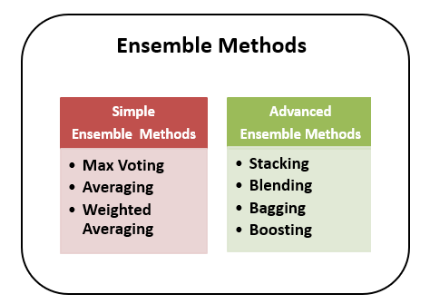
Types of Ensemble Methods
1. Simple Ensemble Methods
Max Voting
Each model votes for a class, and the class with the most votes wins. It is used mainly for classification. If three models predict spam, not spam and spam, the ensemble answers spam. This is also called hard voting. If votes are tied, the result depends on the library, so it is best to use an odd number of models.
Averaging
Each model produces a number, and the ensemble takes the average. For regression, the numbers are predictions. For classification, they can be predicted probabilities, which is called soft voting. Averaging smooths out the quirks of individual models.
Weighted Average
Some models deserve more trust than others. A weighted average gives stronger models a larger say. The following example uses predicted probabilities for three classes from three models.
| Model | Class 1 | Class 2 | Class 3 |
|---|---|---|---|
| Model 1 | 0.2 | 0.5 | 0.3 |
| Model 2 | 0.6 | 0.3 | 0.1 |
| Model 3 | 0.3 | 0.4 | 0.3 |
| Equal weights average | 0.37 | 0.40 | 0.23 |
| Weights 2, 5 and 1 | 0.46 | 0.36 | 0.18 |
With equal weights, class 2 wins with 0.40. But if Model 2 is the most trustworthy and gets a weight of 5, with weights of 2 and 1 for the others, class 1 wins with about 0.46. The data did not change, only the trust. That is why choosing weights matters, and why they should be chosen on validation data, not by hunch.
2. Advanced Ensemble Methods
Stacking
Stacking lets a model learn how to combine the others. The base models make predictions, and those predictions become the input features of a final model, sometimes called the meta model. The final model learns, for example, that Model 1 is reliable for some kinds of cases and Model 2 for others.
There is one trap. If the base models predict on the same rows they were trained on, their predictions look too good, and the final model learns to trust them too much. To avoid this, stacking uses predictions made on data the base models did not train on, produced by cross validation. Scikit learn does this for you inside StackingClassifier.
Blending
Blending is a simpler cousin of stacking. Instead of cross validation, you set aside a validation set, usually 10 to 20 percent of the training data. The base models are trained on the rest, they predict on the validation set, and the final model is trained on those predictions.
| Point | Stacking | Blending |
|---|---|---|
| Final model trained on | Cross validated predictions for every training row | Predictions on one held out validation set |
| Data used | All the training data | Less, because some is held out |
| Complexity | More, and slower | Simpler and faster |
| Leakage risk | Handled by cross validation | Low, if the split is kept separate |
| In scikit learn | StackingClassifier and StackingRegressor | No ready made class, write it by hand |
Bagging
Bagging, short for bootstrap aggregating, trains many models in parallel, each on a random sample of the data drawn with replacement, and averages them. It reduces variance and works best with strong, unstable models such as deep decision trees. Random forest is bagging plus a random choice of features at each split. Our full guide to bagging covers it in detail.
Boosting
Boosting trains simple models in sequence. Each new model concentrates on the mistakes of the ones before it, and the final prediction combines them all. It reduces bias and often gives the highest accuracy on tables of data. AdaBoost, gradient boosting, XGBoost, LightGBM and CatBoost are all boosting methods. Our full guide to boosting covers them.
Bagging Versus Boosting
| Point | Bagging | Boosting |
|---|---|---|
| Main goal | Reduce variance | Reduce bias |
| Build order | Independent, in parallel | In sequence |
| Best base models | Strong and complex | Weak and simple |
| Overfitting risk | Low | Higher if run too long |
| Typical choice when | Your model is accurate but unstable | Your model is too simple and underfits |
Ensemble Methods in Python
Here is a complete program that compares three individual models against hard voting, soft voting and stacking. All use the same training and test split of the breast cancer dataset that comes with scikit learn.
from sklearn.datasets import load_breast_cancer
from sklearn.model_selection import train_test_split
from sklearn.pipeline import make_pipeline
from sklearn.preprocessing import StandardScaler
from sklearn.linear_model import LogisticRegression
from sklearn.ensemble import RandomForestClassifier, VotingClassifier, StackingClassifier
from sklearn.naive_bayes import GaussianNB
X, y = load_breast_cancer(return_X_y=True)
X_train, X_test, y_train, y_test = train_test_split(
X, y, test_size=0.3, random_state=0, stratify=y
)
lr = make_pipeline(StandardScaler(), LogisticRegression(max_iter=1000))
rf = RandomForestClassifier(n_estimators=100, random_state=0)
nb = GaussianNB()
base = [(“lr”, lr), (“rf”, rf), (“nb”, nb)]
models = {
“Logistic regression”: lr,
“Random forest”: rf,
“Naive Bayes”: nb,
“Hard voting”: VotingClassifier(base, voting=”hard”),
“Soft voting”: VotingClassifier(base, voting=”soft”),
“Stacking”: StackingClassifier(base, final_estimator=LogisticRegression(max_iter=1000), cv=5),
}
for name, model in models.items():
model.fit(X_train, y_train)
print(f”{name}: {model.score(X_test, y_test):.3f}”)
When I ran it, the output was:
Logistic regression: 0.959
Random forest: 0.953
Naive Bayes: 0.924
Hard voting: 0.959
Soft voting: 0.942
Stacking: 0.971
Reading the Results
- Stacking did best. It scored 0.971, against 0.959 for the best single model.
- Voting did not always help. Hard voting only matched the best single model, and soft voting scored lower than logistic regression. The weakest member, Naive Bayes, may have dragged it down.
- The differences are small. The test set has 171 patients, and each patient is worth about 0.6 points. Stacking’s lead is two patients. Treat these results as a demonstration, and use cross validation on your own data before drawing conclusions.
The lesson matters more than the numbers. An ensemble is not guaranteed to beat its best member. It helps most when the members are individually good and make different kinds of mistakes.
How to Choose an Ensemble Method?
| Your situation | Try first |
|---|---|
| A deep tree is accurate but unstable | Bagging or random forest |
| Your model underfits and is too simple | Boosting |
| You have a few good, different models already | Voting or stacking |
| You have a small dataset and little time | Random forest |
| You want the highest accuracy on tabular data | Gradient boosting, then consider stacking |
| You want to keep it simple and explainable | A single model, or a small voting ensemble |
Strengths and Limitations of Ensembles
Strengths
- Usually more accurate and more stable than one model.
- Reduce the chance of one bad model ruining results.
- Work with almost any type of base model.
Limitations
- Slower to train and to predict.
- Harder to explain than a single model.
- More code and more settings to maintain.
- Gains can be small if the models make the same mistakes.
Common Mistakes to Avoid
- Combining models that are too similar. If they all make the same errors, nothing cancels.
- Training stacking models on their own training predictions. Use cross validation, which StackingClassifier does for you.
- Choosing weights by hunch. Pick them on validation data.
- Expecting an ensemble to win every time. It does not.
- Evaluating on the training set. Always keep a held out test set.
- Ignoring cost. An ensemble of fifty models may not be worth a half point of accuracy in production.
Ensemble methods turn many imperfect models into one stronger one. Start by running the comparison program on your own data, check whether combining actually helps, and pick between bagging, boosting, voting and stacking based on what your single model gets wrong.
