Naive Bayes Classifier in Machine Learning
Naive Bayes Classifier in Machine Learning
Every day your email inbox decides, in a fraction of a second, whether a message is spam. It does not read the message the way you do. It looks at the words, asks how often each one appears in spam compared with normal mail, and combines those clues into a single judgement. One of the oldest and most successful ways to do that is the Naive Bayes classifier.
Naive Bayes is a classification method built on a result from probability called Bayes theorem. Despite a deliberately simple assumption, it is fast, needs little training data and works surprisingly well on text problems such as spam filtering, sentiment analysis and document sorting. That is why it is often the first model people try, and a sensible baseline to beat.
This guide builds the idea from the ground up. We start with Bayes theorem and why the method is called naive, then work through a full example by hand so you can see every number. After that comes Gaussian Naive Bayes for continuous data with a working Python program, the other variants, smoothing, strengths and limits, applications, common mistakes and a short FAQ.
Introduction to Bayes Theorem
Bayes theorem tells you how to update a belief when you see new evidence. It connects two questions that sound similar but are not the same: how likely is the evidence if the thing is true, and how likely is the thing to be true given the evidence.
P(A given B) = P(B given A) * P(A) / P(B)
- P(A given B)is the probability of A once you know B has happened. This is what we want.
- P(B given A)is the probability of seeing B if A is true. It is called the likelihood.
- P(A)is how likely A is before seeing anything. It is called the prior.
- P(B)is how likely the evidence is overall.
Here is a small example. Suppose 20 percent of your email is spam. The word offer appears in 60 percent of spam but only 5 percent of normal mail. An email arrives containing offer. How likely is it to be spam?
Spam and offer: 0.60 * 0.20 = 0.12
Not spam and offer: 0.05 * 0.80 = 0.04
P(spam given offer) = 0.12 / (0.12 + 0.04) = 0.75
A 20 percent prior turned into a 75 percent probability after one piece of evidence. That is Bayes theorem at work.
Why is It Called Naive?
A real email has many words, not one. Doing the exact calculation with all of them would need to know how every word combination behaves together, which needs far more data than anyone has. Naive Bayes takes a shortcut. It assumes that, once you know the class, each feature is independent of the others. So it simply multiplies the clues together.
That assumption is almost never exactly true. Words like free and offer often appear together. But the method is still often accurate, because it only needs to rank the classes correctly and not to get every probability right. The assumption is the naive part, and it is also what makes the method so cheap to train.
One correction to a common misreading: this does not mean every feature gets the same weight. Features with stronger evidence move the answer more. It means the features are treated as independent given the class.
Naive Bayes Classifier Example
Imagine you want to predict whether a cricket match will be played, based on the weather. Here are 14 past days. The first four columns are the features, collected into a feature matrix. The last column is the response, the thing we want to predict, collected into a response vector.
| Outlook | Temperature | Humidity | Windy | Cricket played |
|---|---|---|---|---|
| Sunny | Hot | High | No | No |
| Sunny | Hot | High | Yes | No |
| Overcast | Hot | High | No | Yes |
| Rainy | Mild | High | No | Yes |
| Rainy | Cool | Normal | No | Yes |
| Rainy | Cool | Normal | Yes | No |
| Overcast | Cool | Normal | Yes | Yes |
| Sunny | Mild | High | No | No |
| Sunny | Cool | Normal | No | Yes |
| Rainy | Mild | Normal | No | Yes |
| Sunny | Mild | Normal | Yes | Yes |
| Overcast | Mild | High | Yes | Yes |
| Overcast | Hot | Normal | No | Yes |
| Rainy | Mild | High | Yes | No |
The Two Assumptions
- Conditional independence.Given whether cricket is played, the weather features do not influence each other.
- Every feature contributes.All the features are used as evidence, though not all push equally hard.
How Naive Bayes Works, Step by Step
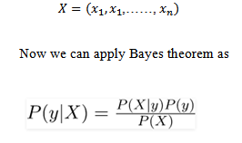
New day to predict: Sunny, Mild, Normal humidity, not windy. Will cricket be played? For each answer, Yes and No, we multiply a prior by the likelihood of each feature, then compare.
Step 1: the priors. Cricket was played on 9 of the 14 days and not played on 5.
P(Yes) = 9/14 = 0.643
P(No) = 5/14 = 0.357
Step 2: the likelihoods for Yes. Among the 9 days when cricket was played, count how often each feature value appeared.
P(Sunny | Yes) = 2/9
P(Mild | Yes) = 4/9
P(Normal | Yes) = 6/9
P(Not windy | Yes) = 6/9

Step 3: the likelihoods for No. Do the same for the 5 days when cricket was not played.
P(Sunny | No) = 3/5
P(Mild | No) = 2/5
P(Normal | No) = 1/5
P(Not windy | No) = 2/5

Step 4: multiply and compare.
Score(Yes) = 0.643 * 0.222 * 0.444 * 0.667 * 0.667 = 0.0282
Score(No) = 0.357 * 0.600 * 0.400 * 0.200 * 0.400 = 0.0069
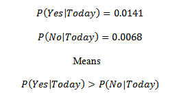
Yes scores higher. To turn the scores into probabilities, divide each by their total. That gives about 80.5 percent for Yes and 19.5 percent for No. Naive Bayes predicts that cricket will be played.
The Zero Frequency Problem and Smoothing
What if a feature value never appeared with a class in your training data? Its likelihood would be zero, and because we multiply, one zero wipes out the whole score. The fix is smoothing. Add a small count, usually 1, to every feature value so nothing is ever exactly zero. Adding 1 is called Laplace smoothing. In scikit learn, the setting is called alpha.
Gaussian Naive Bayes Classifier
The weather example uses categories. What about measurements such as height, temperature in degrees or a blood test value? Gaussian Naive Bayes handles continuous features by assuming that, within each class, each feature follows a bell shaped normal distribution. For every class it learns the average and the spread of each feature.
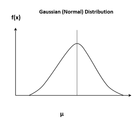
The probability of a feature value x for a class y is then read off the bell curve:
P(x | y) = 1 / sqrt(2 * pi * sigma_y^2) * exp( -(x – mu_y)^2 / (2 * sigma_y^2) )
Here mu_y is the average of the feature in class y, and sigma_y is its standard deviation.

Gaussian Naive Bayes in Python
We will use the breast cancer dataset that comes with scikit learn, which has 30 measurements for each of 569 tumours and a label for malignant or benign. This complete program loads the data, splits it, trains the model and checks the accuracy.
from sklearn.datasets import load_breast_cancer
from sklearn.model_selection import train_test_split
from sklearn.naive_bayes import GaussianNB
from sklearn.metrics import accuracy_score
X, y = load_breast_cancer(return_X_y=True)
X_train, X_test, y_train, y_test = train_test_split(X, y, test_size=0.25, random_state=0)
model = GaussianNB()
model.fit(X_train, y_train)
y_pred = model.predict(X_test)
print(“Accuracy:”, round(accuracy_score(y_test, y_pred) * 100, 2), “percent”)
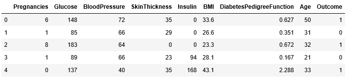
Running it prints:
Accuracy: 93.71 percent
A model trained in a fraction of a second gets about 94 percent of the test cases right, which is a respectable result for a baseline. If you also want the probabilities, call predict_proba, but see the warning below before you trust them.
Types of Naive Bayes Classifiers
| Variant | Feature type | Best suited for |
|---|---|---|
| GaussianNB | Continuous numbers | Measurements that look roughly bell shaped |
| MultinomialNB | Counts | Text classification using word counts or tf idf |
| ComplementNB | Counts | Imbalanced text data, often better than MultinomialNB |
| BernoulliNB | Yes or no features | Word present or absent, shorter documents |
| CategoricalNB | Categories | Data like the weather table, encoded as numbers first |
Strengths and Limitations of Naive Bayes
Strengths
- Fast to train and fast to predict.
- Needs only a small amount of training data.
- Copes well with a very large number of features, such as words.
- Works well on text problems like spam filtering.
- Simple to explain, since you can read off which features pushed the answer.
Limitations
- The independence assumption is rarely true, so strongly related features are double counted.
- The probability scores are unreliable.scikit learn itself notes that Naive Bayes is a decent classifier but a poor estimator, so the output of predict_proba should not be taken too seriously without calibration.
- Gaussian Naive Bayes expects roughly bell shaped features and can struggle otherwise.
- It cannot learn interactions between features.
Applications of Naive Bayes
- Spam filtering. Classifying email from word evidence.
- Sentiment analysis. Deciding whether a review is positive or negative.
- Document and news classification. Sorting text by topic.
- Recommendation and ranking. Quick first stage classifiers.
- Medical screening. Combining test results into a risk estimate.
- Real time prediction. The speed suits systems that must answer instantly.
Common Mistakes to Avoid
- Saying all features have equal weight. The assumption is independence, not equal weight.
- Trusting the probabilities. Use the predicted class, and calibrate if you need real probabilities.
- Forgetting smoothing. One unseen value can zero out a prediction.
- Using the wrong variant. Use Gaussian for continuous values, Multinomial for counts and Bernoulli for yes or no.
- Evaluating on the training data. Always check accuracy on a held out test set.
- Pasting code with curly quotes. Paste into a plain editor first.
Naive Bayes proves that a simple idea can go a long way. Work through the weather table by hand once, run the Python program, and then try a text dataset with MultinomialNB. Treat it as the baseline that every fancier model has to beat.
