Principle Component Analysis Tutorial
Principal Component Analysis Tutorial
Principal Component Analysis Tutorial, in this Tutorial one, can learn types of principal component analysis. Are you the one who is looking for the best platform which provides information about know working principle of PCA, Applications of Principal Component Analysis? Or the one who is looking forward to taking the advanced Data Science Certification Course with Machine Learning from India’s Leading Data Science Training institute? Then you’ve landed on the Right Path.
With the advancements within the field of Machine Learning and computer science, it’s become essential to grasp the basics behind such technologies. This blog on Principal Component Analysis will facilitate your understanding of the concepts behind dimensionality reduction and the way it may be wont to house high-dimensional data.
The Below mentioned Principal Component Analysis Tutorial will help to Understand the detailed information about what is PCA in machine learning, so Just follow all the tutorials of India’s Leading Best Data Science Training institute in Bangalore and Be a Pro Data Scientist or Machine Learning Engineer.
What is PCA in Machine Learning?
Suppose you have to deal with the dataset based on GDP (Gross Domestic Production) of any country. While processing on data you will come across so many fields, which we call as features or variables. Now the question arises, how we can take all variables and select only a few of them for further processing? There may be a problem of overfitting the model. So we have to reduce the dimensionality of that data so that it will be easier and we can have a smaller amount of relationships between variables to consider. So, reducing dimensions of feature space is nothing but ‘Dimensionality Reduction.
Types of Principal Component Analysis
There are different methods to achieve dimensionality reduction. Mostly used methods are categorized into:
Features Elimination
Features Extraction
Feature Elimination
As the name suggests, in this method the features are eliminated which are having very low significance. Here only the best features are selected as per domain requirement. The rest features are eliminated. Simplicity and maintaining interpretability are the advantages of variables in this method.
Feature Extraction
Suppose we have N number of independent variables. In feature extraction, we create N “new” independent variables, where each newly generated independent variable is a combination of each of the N “old” independent variables. However, the newly created variables have arranged in a specific order based on how well they predict the dependent variable. While following these methods, we always eliminate or remove the features which are ‘least important’. And there ‘Dimensionality reduction’ comes in a picture. As we ordered the new variables by how well they predict our dependent variable, we are well known about which variable is the most important and least important. Still, we are keeping the most valuable parts of our old variables, even when we drop one or more of these “new” variables.
When PCA can be used?
If we want to reduce the number of variables, but we are unable to identify which variables to completely remove from consideration then PCA is the best option. Even, there are some cases where we can make independent variables less interpretable and we have to ensure those variables are independent of each other also.
Principal Component Analysis (PCA) is a numerical procedure that uses an orthogonal alteration. It converts a set of correlated variables to a set of uncorrelated variables. Investigative data analysis and predictive models use PCA as an effective tool. It is also called general factor analysis, as a line of best fit is determined by regression.
Working Principle of PCA
In simple words, PCA takes a dataset with a lot of dimensions and flattens it to 2 or 3 dimensions. It tries to find a meaningful way to flatten the data by focusing on the things that are different between independent variables.
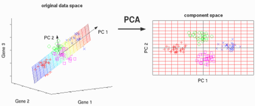
The image above shows the example of a transformation of high-dimensional data i.e. 3-dimensional data to low dimensional i.e. 2-dimensional data using PCA. Before moving to the actual concept, let’s see some terminologies related to PCA.
Dimensionality: It is simply the number of features or the number of columns present in our dataset. We can consider it as a number of random variables in a dataset
Correlation: It displays how strongly two variables are related to each other. The value ranges from -1 to +1. Positive indicates that if one variable increases, the other will increase as well, while negative indicates the other decreases on increasing the other. And the modulus value indicates the strength of the relation.
Orthogonal: Uncorrelated to every other, i.e., a correlation between any pair of variables is 0.
Eigenvectors: Let’s consider a non-zero vector v. Let’s take a square matrix A. So it is an eigenvector of a A, if Av is a scalar multiple of v. Or simply:
Av = ƛv
Here, v is the eigenvector
ƛ is the eigenvalue associated with it.
Covariance Matrix: This matrix consists of covariance between the pairs of variables. The covariance between i-th and j-th variable is nothing but this (i,j)th element.
Principal Components
A normalized linear combination of the original predictors in a data set is called a principal component is. In the image above, the principal components are indicated by PC1 and PC2. We can fit the data into two axes, which are nothing but these principle components i.e. PCs.
PC1 is the first principle axis that spans the most variation, whereas PC2 is the second principal axis which spans the second most variation. Means PC1 will capture the directions where most of the variation is present and PC2 captures the direction with the second-most variation.
The PCs are essentially the linear combinations of the original variables, the weights vector in this combination is actually the eigenvector found which in turn satisfies the principle of least squares.
The PCs are orthogonal in nature.
As we move from the 1st PC to the last one, the variation present in PCs decreases.
Sometimes in regression, outlier detection problems, these least important PCs are useful.
Implementing PCA on a 2-D Dataset
Step 1: Normalize the data:
The first step is to normalize data that we have so that PCA works properly. This is done by subtracting respective means from numbers in the respective column. Let’s consider we have two dimensions X and Y. All X will be ?- and all Y will be ?-. This produces a dataset whose mean is zero.
Step 2: Calculate the covariance matrix
Since the dataset we took is 2-dimensional, this will give result in a 2×2 Covariance matrix.
Please note that
Var[X1] = Cov[X1,X1]
Var[X2] = Cov[X2,X2].
Step 3: Calculate the eigenvalues and eigenvectors:
The next step is to calculate eigenvalues and eigenvectors for the covariance matrix. For a matrix A, ƛ is an eigenvalue which is a solution of the characteristic equation:
det( ƛI – A ) = 0
Where,
It is the identity matrix of the same dimension as matrix A. It is a required condition for matrix subtraction.
‘det’ is the determinant of the matrix.
For each eigenvalue ƛ, a corresponding eigenvector v can be found by solving:
( ƛI – A )v = 0
Step 4: Selecting components and forming a feature vector:
We order eigenvalues from largest to smallest so that it gives us components in order or significance. Here comes the dimensionality reduction part. If we have data with n variables, then we have corresponding n eigenvalues and eigenvectors. It turns out that the eigenvector corresponding to the highest eigenvalue is the principal component of the dataset and it is our call as to how many eigenvalues we choose to move ahead of our analysis with. To reduce dimensions, we choose the first p eigenvalues and ignore rest. We do lose out some information in the process, but if eigenvalues are small, we do not lose much.
Next, we will form a feature vector which is a matrix. This is a matrix of vectors with the eigenvectors which we want to proceed with. Since we have just 2 dimensions in the running example, we can either choose one corresponding to greater eigenvalue or simply take both.
Feature Vector = (eig1, eig2)
Step 5: Forming Principal Components
This is the final step where we actually form principal components using all math we did till here. For the same, we take the transpose of the feature vector and left-multiply it with the transpose of a scaled version of the original dataset.

Here,
NewData = Matrix consisting of the principal components,
Feature Vector = matrix we formed using eigenvectors we chose to keep, and
Scaled Data is a scaled version of the original dataset
Where T denotes the transpose of matrices.
If we go back to the theory of eigenvalues and eigenvectors, we will see that, essentially, eigenvectors provide us with information about patterns in data. In this example, if we plot eigenvectors on a scatterplot of data, we find that the principal eigenvector actually fits well with data. The other one, being perpendicular to it, does not carry much information, and hence, we are at not at much loss when deprecating it, hence reducing the dimension.
All the eigenvectors of a matrix are orthogonal i.e. perpendicular to each other. So, in PCA, what we do is represents or transforms the original dataset using these orthogonal (perpendicular) eigenvectors instead of representing on the normal x and y axis. We have now classified our data points as a combination of contributions from both x and y. The difference lies when we actually disregard one or many eigenvectors, hence, reducing the dimension of the dataset. Otherwise, in case, we take all eigenvectors into an account, we are just transforming coordinates and hence, not serving a purpose.
Applications of Principal Component Analysis
PCA is predominantly used as a type of a dimensionality reduction technique in domains like facial recognition, computer vision, and image compression. It is also used for determining patterns in data of high dimension in fields of finance, data mining, bioinformatics, psychology, etc.
Step by Step Implementation of PCA using Python
Import required libraries
%matplotlib inline
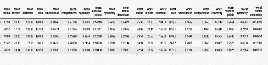
Import dataset
from sklearn.datasets import load_breast_cancer
cancer=load_breast_cancer()
df=pd.DataFrame(cancer[‘data’],columns=cancer[‘feature_names’])
df.head()
Normalize DataSet using Standard Scalar
from sklearn.preprocessing import StandardScaler
scl= StandardScaler()
scl.fit(df)
scl_data=scl.transform(df)
from sklearn.decomposition import PCA
pca=PCA(n_components=2)
pca.fit(scl_data)
x_pca=pca.transform(scl_data)
x_pca.shape
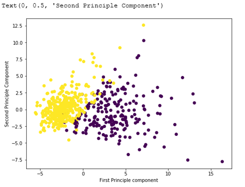
Import and implement PCA
#a larger plot
plt.figure(figsize=(8,6))
plt.scatter (x_pca[:,0],x_pca[:,1],c=cancer[‘target’],cmap=’viridis’)
# Labeling to axes
plt.xlabel(‘First Principle component’)
plt.ylabel(‘Second Principle Component’)
Output:
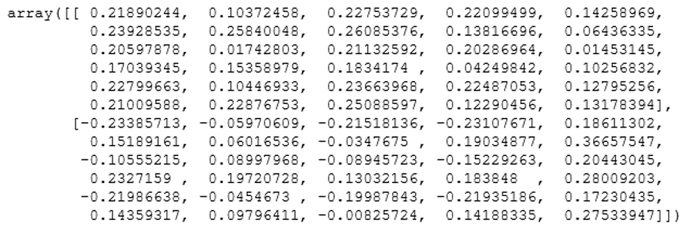
Display Dimension reduced
pca.components_
Output:
We hope you understand Principal Component Analysis Tutorial. Get success in your career as a Data Scientist by being a part of the Prwatech, India’s leading Data Science training institute in Bangalore.