Support Vector Machine Tutorial
Support Vector Machine Tutorial for Beginners
Support Vector Machine Tutorial for Beginners, Are you the one who is looking forward to knowing about What is Support Vector Machine?? Or the one who is looking forward to knowing How does SVM work? and implementing svm in python or Are you dreaming to become to certified Pro Machine Learning Engineer or Data Scientist, then stop just dreaming, get your Data Science certification course with Machine Learning from India’s Leading Data Science training institute.
Support Vector Machine is another simple algorithm that every machine learning expert uses. It is highly preferred by many experts because it provides accurate results with less computation power and is used for both classification and regression problems. In this blog, we will learn How does SVM work in Machine Learning and implementing svm in python. Do you want to know What is Support Vector Machine, So follow the below mentioned support vector machine tutorial for beginners from Prwatech and take advanced Data Science training with Machine Learning like a pro from today itself under 10+ Years of hands-on experienced Professionals.
Introduction to Support Vector Machine
Certainly! Here’s your content with improved coherence and the addition of transition words:
Support Vector Machine (SVM)
Support Vector Machine (SVM) stands as a supervised machine learning algorithm, functioning akin to a discriminative classifier defined by a separating hyperplane. Essentially, for labeled training data, the algorithm constructs the optimal hyperplane, enabling the categorization of new inputs. In two dimensions, this hyperplane manifests as a line that partitions the space into two distinct regions.
Support Vectors
Support Vectors denote the coordinates of unique observations essential for defining the separating hyperplane.
How Support Vector Machine Works
Support Vector Machine (SVM) operates by identifying the optimal hyperplane to separate two classes of data points. Despite the existence of multiple hyperplanes capable of achieving this, SVM aims to select the one with the maximum margin. This margin refers to the distance between the hyperplane and the closest data points from each class. By maximizing this margin, SVM strives to enhance generalization and classification performance.
Choosing the Optimal Hyperplane in SVM
Selecting the optimal hyperplane in SVM involves considering various factors. Despite the availability of numerous potential hyperplanes, the primary criterion is to choose the one with the maximum margin. This entails identifying the hyperplane that maintains the greatest distance from the nearest data points of each class. By adhering to this principle, SVM ensures robust and accurate classification outcomes.
This approach enhances the model’s ability to generalize well to unseen data and effectively classify new instances.
Criterion 1
The following image shows three hyperplanes trying to separate out two classes.
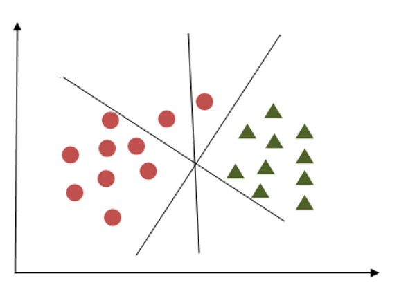
Here we have to choose that hyperplane which segregates two classes. We can see hyperplane X fulfills this criterion.
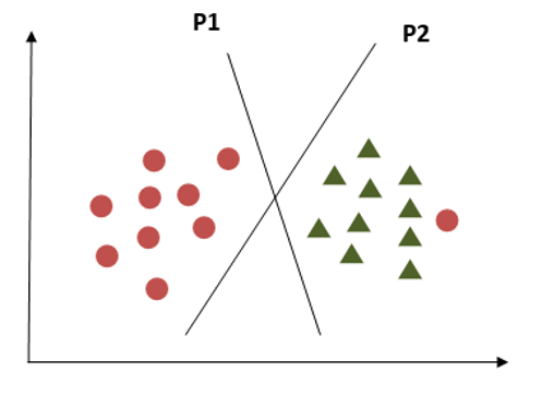
Criterion 2
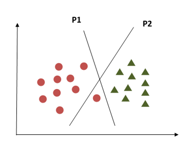
Here all hyperplanes are separating two classes, now the question is how to identify the correct one?

Here we have to consider the maximum distance between the nearest data points in both classes and the hyperplane. This distance is called ‘Margin’. In the above diagram plane, P1 is having maximum distance from the nearest points in both classes.
Criterion 3
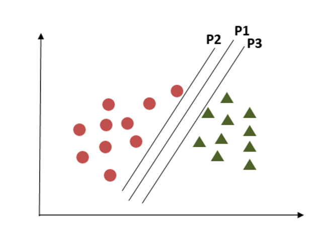
In this criterion, if we choose hyperplane P2 according to a higher margin than P1, it misclassified the data points. So, hyperplane P2 has classification errors but hyperplane P1 can classify correctly.
Criterion 4:
What if the classes are distributed as shown in the above diagram? SVM has a property to ignore the outliers. It is a robust algorithm in case of outliers.
Criterion 5:
Now how to handle this criterion, this is a challenge in using a single line as a hyperplane. SVM handles this problem by using additional features. It can use third plane Z, besides X and Y planes having equation like
z = x^2+y^2
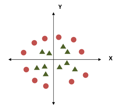
AS we plot the data points across X-Z planes we get the above diagram which clearly shows the segregation of two classes. SVM can handle the separation of different types of data points with appropriate hyperplanes. In the SVM model some parameters are required defined to be tuned for efficient working of that model.
Tuning Parameters: Kernel
The kernel parameter is a crucial factor that determines the nature of the hyperplane in Support Vector Machine (SVM). It plays a pivotal role in the model’s design, offering various options for constructing the hyperplane.
In the case of the Linear Kernel, the prediction equation for a new data point involves the dot product between the input (x) and each support vector (Xi):
f(x) = B(0) + sum(ai * (x,Xi))
The equation calculates the inner products of a new input vector x with all support vectors in training data. B0 and ai coefficients for, each input, must be assessed from the training data by learning algorithm. The polynomial kernel can be written as
K(x,xi) = 1 + sum(x * Xi)^d
And exponential can be written as
K(x,xi) = exp(-gamma * sum((x — xi²))
Understanding Regularization in SVM
The regularization parameter, often denoted as parameter ‘C’ in the scikit-learn library, plays a crucial role in Support Vector Machine (SVM) optimization. It determines the extent to which misclassification is tolerated during the SVM training process.
When ‘C’ takes on greater values, the optimizer tends to select a smaller-margin hyperplane if it results in better classification of all training points. Conversely, when ‘C’ is set to smaller values, the optimizer prioritizes selecting a larger-margin separating hyperplane, even if it leads to misclassification of some points.
This balancing act between margin size and misclassification is pivotal in ensuring optimal SVM performance and generalization ability.
The first image shows the case of lower regularization where chances of misclassifications are more. In second image high regularization will help to classify data points correctly compared to the first case.
Gamma
The gamma parameter defines how far the impact of a single training point reaches, with low values (meaning ‘far’) and high values (meaning ‘close’). In other words, with low gamma, points far away from reasonable separation line are taken in the calculation for the separation line. And in case of higher gamma value, the points close to the plausible line are taken in the calculation.
Margin
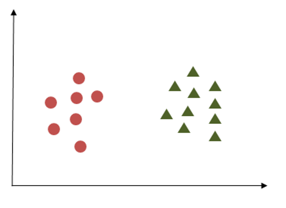
Understanding Margin in Support Vector Machine (SVM)
A margin in Support Vector Machine (SVM) refers to the separation of the decision boundary (hyperplane) from the nearest points of the classes it is intended to separate. In essence, a good margin entails a substantial separation for both classes, allowing data points to reside comfortably within their respective classes without encroaching on the boundaries of other classes.
This spacious margin not only facilitates clearer class separation but also enhances the model’s robustness and generalization ability. Let’s delve into an example to illustrate this concept.
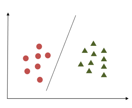
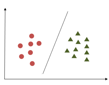
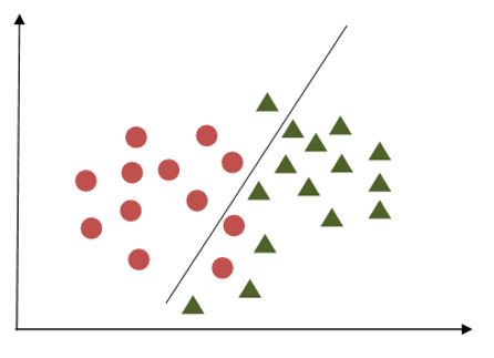
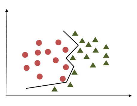
Support Vector Machine Example
In the first example, the margin appears inadequate as it closely aligns with the points belonging to the first class, depicted as circles. Conversely, in the second example, the margin is more substantial, maintaining a greater distance from the nearest points in both classes.
Now, let’s delve into how we can implement SVM in Python and explore the effects of different parameters on the results. To do this, we will utilize a dataset from the scikit-learn library.
Initializing and importing required libraries
import NumPy as np
import matplotlib.pyplot as plt
from sklearn import svm, datasets
Let’s take the iris data set and load it. We will check features in iris and we will select two features from them to avoid complex visualization.
iris = datasets.load_iris()
print(iris.feature_names)
Xin = iris.data[:, :2] # we will take ‘sepal width’ and ‘sepal length’.
yin = iris.target
We will try to plot support vectors using linear kernel, polynomial kernel, and sigmoid kernel. For this we will keep C and gamma values constant.
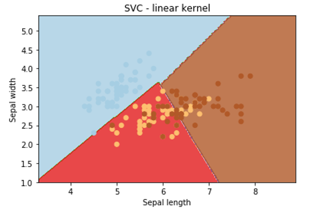
Let’s apply the linear kernel first:
C = 1.0 # Support Vector Machine regularization parameter
svc = svm.SVC(kernel=’linear, C=1,gamma=’auto’).fit(X, y)
x_min, x_max = Xin[:, 0].min() – 1, Xin[:, 0].max() + 1
y_min, y_max = Xin[:, 1].min() – 1, Xin[:, 1].max() + 1
h = (x_max / x_min)/100
x1, y1 = np.meshgrid(np.arange(x_min, x_max, h),np.arange(y_min, y_max, h))
plt.subplot(1, 1, 1)
Z = svc.predict(np.c_[x1.ravel(), y1.ravel()])
Z = Z.reshape(x1.shape)
plt.contourf(x1, y1, Z, cmap=plt.cm.Paired, alpha=0.8)
plt.scatter(Xin[:, 0], Xin[:, 1], c=yin, cmap=plt.cm.Paired)
plt.xlabel(‘Sepal length’)
plt.ylabel(‘Sepal width’)
plt.xlim(x1.min(), x1.max())
plt.title(‘SVC – linear kernel’)
plt.show()
Output:
Now we have to see the results of different kernels. By keeping rest code similar we have to just change the type of kernel as follows
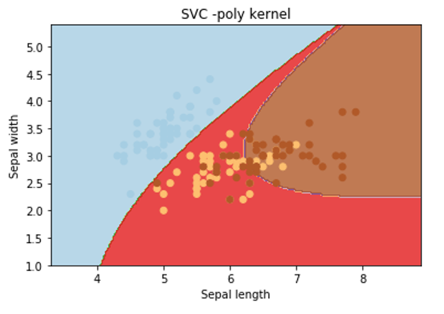
Let’s apply poly kernel:
svc = svm.SVC(kernel=’poly’, C=1,gamma=’auto’).fit(X, y)
Output:
Let’s apply rbf kernel:
svc = svm.SVC(kernel=’rbf’, C=1,gamma=’auto’).fit(X, y)
Output:
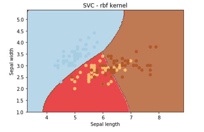
From the above graphical representation, it is clearly observed that change in the kernel will change the contour in the image and try to classify data points in a different manner to approach the correct classification.
Now Let’s observe the effect of ‘gamma’ on classification. For that, we will keep the SVM kernel and C constant.
If we change values of gamma as 1,10,200 then we get the respective graph as follows:
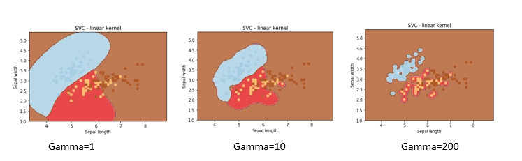
Now, let’s delve into the effect of the parameter ‘C’ on classification outcomes. In this analysis, we’ll keep gamma and the SVM kernel constant to isolate the influence of ‘C’ on the classification process.
If we change values of C as 5,500,5000 then we get the respective graph as follows:
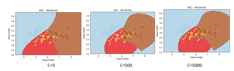
We hope you understand the support vector machine tutorial for beginners. Get success in your career as a Data Scientist by being a part of the Prwatech, India’s leading Data Science training institute in Bangalore.