Support Vector Machine Tutorial
Support Vector Machine Tutorial for Beginners
Imagine two groups of houses on opposite sides of a river, and you need to draw a fence that separates them. You could draw it anywhere in the gap, but some fences are better than others. A fence that hugs one group is risky, because a new house built a little off the pattern ends up on the wrong side. The safest fence runs down the middle of the widest empty space. That is the whole idea behind the support vector machine.
A support vector machine, or SVM, is a supervised learning algorithm used mainly for classification. It looks for the boundary that separates classes with the largest possible gap on both sides. That gap is called the margin, and the data points that touch it are called support vectors. A wide margin gives a model that tends to cope well with new data, which is why SVMs became one of the most trusted algorithms for problems with small and medium sized datasets and many features, such as text and gene data.
This tutorial starts from the plain picture and builds up. You will learn what a hyperplane is, how the margin and the support vectors work, and how SVM chooses between several possible boundaries. Then comes the part that makes SVM powerful: the kernel trick, which lets it separate data that no straight line can divide. We cover the two settings that matter most, C and gamma, and finish with a complete Python program using scikit learn that was run and checked, plus common mistakes and a short FAQ.
What is a Support Vector Machine?
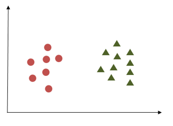
In a two class problem, SVM finds a boundary between the classes. With two features, that boundary is a line. With three features it is a flat plane. With more features it is called a hyperplane, which is simply the same idea in higher dimensions. A new point is classified by which side of the hyperplane it falls on.
Many hyperplanes can separate the same data. SVM picks the one with the maximum margin, meaning the largest distance to the nearest point of each class.
What are Support Vectors?
Support vectors are the training points closest to the boundary. They sit right on the edge of the margin, and they alone decide where the hyperplane goes. If you removed every other point, the boundary would not move. If you moved a support vector, the boundary would shift.
This is a useful property. SVM does not need to remember all the data, only the handful of points that matter. In the program later in this tutorial, a model trained on 210 points needed only 67 support vectors.
How Does SVM Work?
The process has a simple logic, which we can follow in four steps.
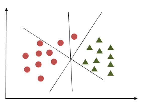
- Draw candidate boundaries. Many lines could split the classes.
- Measure the margin of each. The margin is the distance from the boundary to the nearest point on either side.
- Pick the widest. The boundary with the largest margin is chosen.
- Classify new points. Each new point is labelled by the side of the boundary it lands on.
How to Choose the Right Hyperplane?
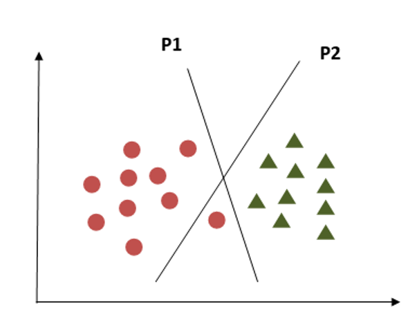
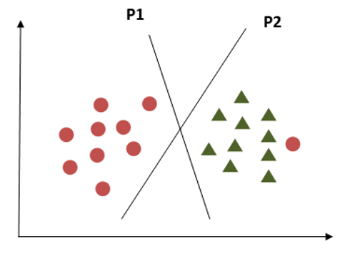
When the choice is not obvious, these five situations show how SVM reasons. Each one has a picture on the original page, which stays in place below.
Criterion 1: Pick the Hyperplane That Separates the Classes Better
If several lines are candidates, the one that splits the two classes more cleanly is the better choice. A line that leaves points of both classes on one side is clearly worse than a line that keeps each class on its own side.
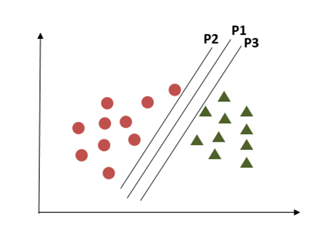
Criterion 2: Maximise the Distance to the Nearest Points
When more than one line separates the classes correctly, choose the one with the largest distance to the nearest point of each class. This distance is the margin. A larger margin means more room for error, so the boundary is more likely to hold up on new data.
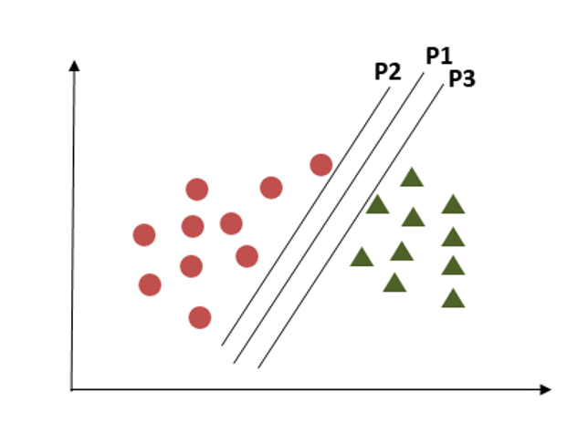
Criterion 3: Classify Correctly Before You Maximise the Margin
A wider margin is not worth it if it misclassifies points. SVM puts correct classification first. It looks for the widest margin only among boundaries that already separate the data well.
Criterion 4: Ignore Outliers When the Data Has Them
Sometimes a single point sits deep inside the other class. A strict boundary would twist itself to catch that point and end up with a tiny margin. SVM can treat such a point as an outlier and ignore it, which keeps the boundary simple and the margin wide. How strict it is about this is controlled by the setting called C, covered below.
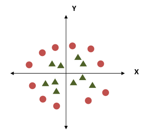
Criterion 5: Add a Dimension When No Straight Line Works
Some data cannot be split by any straight line, for example one class forming a ring around the other. In that case SVM adds a new feature to lift the points into a higher dimension, where a flat boundary can separate them. This is the idea of the kernel trick, explained next.
The Kernel Trick in Plain Words
Take points where one class sits near the center and the other forms a ring around it. No line can separate them on a flat page. Now add a third value for each point, z = x squared plus y squared, which is the squared distance from the center. The inner points get small z values and the outer points get large ones. In three dimensions, a flat sheet at the right height splits them cleanly.
z = x^2+y^2
Computing new features for every point can be expensive. The kernel trick gets the same result without ever building the new features. A kernel function measures how similar two points are as if they were in the higher dimension, and the algorithm needs only that similarity. This is why SVM can work with very complex boundaries at a reasonable cost.
Tuning Parameters of SVM
Kernel
The kernel decides the shape of the boundary. These are the four built in options in scikit learn.
| Kernel | What it does | Use it when |
|---|---|---|
| linear | A straight line or flat plane | Data is roughly separable by a line, or you have many features, as in text |
| poly | A curved boundary of a chosen degree. The formula is gamma times the dot product of the points, plus a constant r, all raised to the power d | You expect interactions between features. Slower, and the degree needs tuning |
| rbf | A smooth, flexible curve. Similarity falls with distance, as exp of minus gamma times the squared distance between points | The safe default when you do not know the shape of the data |
| sigmoid | Based on the tanh function, like a small neural network unit | Rarely. It can behave poorly, so try rbf first |
In practice, start with linear to get a baseline, then try rbf. Choose between them on validation data, not by guess.
Regularization: The C Parameter
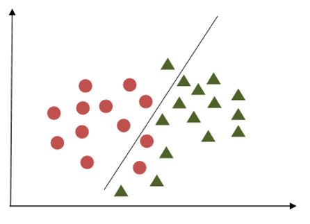
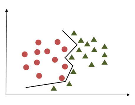
C controls how much SVM is punished for misclassifying training points. It is the balance between a wide margin and a perfect fit.
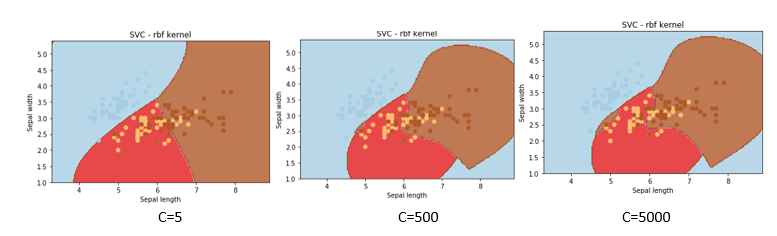
- Low Caccepts a few mistakes in return for a wider, smoother boundary.
- High Ctries hard to classify every training point correctly, which gives a narrower margin and a twisted boundary that can overfit.
The default in scikit learn is 1. Think of C as how strictly the model is graded on its training data.
Gamma
Gamma applies to the rbf, poly and sigmoid kernels. It sets how far the influence of a single training point reaches.
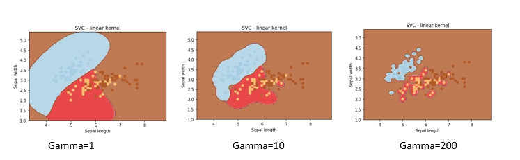
- Low gammameans each point has a far reaching influence, so the boundary is smooth and simple.
- High gammameans each point only affects its close neighbours, so the boundary wraps tightly around individual points and can overfit.
Margin
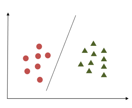
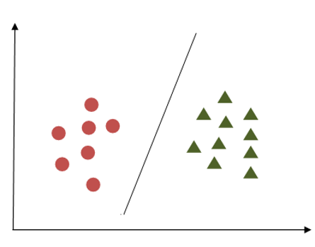
The margin is the output of those settings working together. A good margin leaves a clear gap between the classes on both sides of the boundary. A bad one is too narrow, close to one class, or has points inside it. Always judge it with a held out test set, not by how the training plot looks.
SVM in Python With scikit learn
Here is a full program using two datasets. The first part compares the three main kernels on the Iris flower dataset, which has 150 flowers in 3 species. The second part uses a curved, noisy two class dataset to show what changing gamma and C actually does. The last line counts the support vectors.
Notice that the first part wraps the SVM in a pipeline with a scaler. This matters, and the reason is explained in the next section.
from sklearn.datasets import load_iris, make_moons
from sklearn.model_selection import train_test_split
from sklearn.pipeline import make_pipeline
from sklearn.preprocessing import StandardScaler
from sklearn.svm import SVC
# Part 1: three kernels on the Iris dataset
X, y = load_iris(return_X_y=True)
X_train, X_test, y_train, y_test = train_test_split(
X, y, test_size=0.3, random_state=0, stratify=y
)
for kernel in [“linear”, “poly”, “rbf”]:
model = make_pipeline(StandardScaler(), SVC(kernel=kernel))
model.fit(X_train, y_train)
print(kernel, “kernel test accuracy:”, round(model.score(X_test, y_test), 3))
# Part 2: how gamma and C change the result on curved data
Xm, ym = make_moons(n_samples=300, noise=0.3, random_state=0)
Xm_train, Xm_test, ym_train, ym_test = train_test_split(
Xm, ym, test_size=0.3, random_state=0, stratify=ym
)
print(“gamma train test”)
for gamma in [0.01, 1, 100]:
m = SVC(kernel=”rbf”, gamma=gamma, C=1).fit(Xm_train, ym_train)
print(gamma, round(m.score(Xm_train, ym_train), 3), round(m.score(Xm_test, ym_test), 3))
print(“C train test”)
for C in [0.01, 1, 1000]:
m = SVC(kernel=”rbf”, gamma=1, C=C).fit(Xm_train, ym_train)
print(C, round(m.score(Xm_train, ym_train), 3), round(m.score(Xm_test, ym_test), 3))
# Part 3: support vectors
final = SVC(kernel=”rbf”, gamma=1, C=1).fit(Xm_train, ym_train)
print(“Support vectors per class:”, final.n_support_, “of”, len(Xm_train), “training points”)
Part 1: Three Kernels on Iris
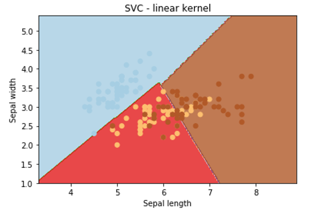
When I ran it, the first part printed:
linear kernel test accuracy: 1.0
poly kernel test accuracy: 0.867
rbf kernel test accuracy: 0.978
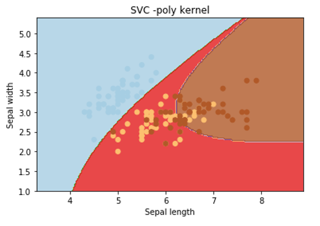
The test set has 45 flowers. The linear kernel classified all of them correctly. The rbf kernel missed one flower. The polynomial kernel missed six, because a curved boundary of this type is more than the Iris data needs. The simple kernel won, which is common on data that is already almost separable.
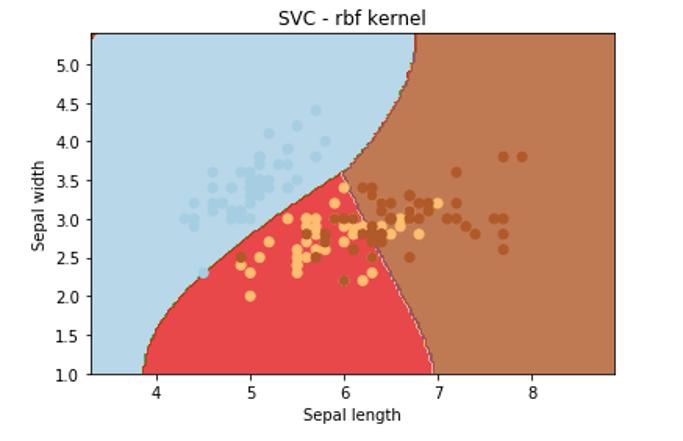
Let’s apply rbf kernel:
svc = svm.SVC(kernel=’rbf’, C=1,gamma=’auto’).fit(X, y)
Output:
Part 2: The Effect of Gamma and C
The second part printed:
gamma train test
0.01 0.843 0.756
1 0.933 0.922
100 0.986 0.922
C train test
0.01 0.857 0.767
1 0.933 0.922
1000 0.948 0.933
| Setting | Train accuracy | Test accuracy | What it shows |
|---|---|---|---|
| gamma 0.01 | 0.843 | 0.756 | Too smooth, underfits |
| gamma 1 | 0.933 | 0.922 | A good balance |
| gamma 100 | 0.986 | 0.922 | Train rises, test does not |
| C 0.01 | 0.857 | 0.767 | Too forgiving, underfits |
| C 1 | 0.933 | 0.922 | A good balance |
| C 1000 | 0.948 | 0.933 | A small gain on test |
- Both extremes at the low end underfit. Test accuracy drops to about 0.76.
- Gamma 100 shows the start of overfitting. Training accuracy climbs to 0.986, but test accuracy stays at 0.922, so the extra fit bought nothing.
- Be careful with small gaps. The test set has only 90 points, and one point is worth about 1.1 points of accuracy. The C 1000 result of 0.933 is one point better than C 1, which is within the noise, not proof that a high C is better.
Part 3: Support Vectors
The last line printed:
Support vectors per class: [32 35] of 210 training points
Only 67 of the 210 training points define the boundary. You can read them from the model with the support_vectors_ attribute, and the count per class with n_support_.
Practical Advice Before You Use SVM
Always Scale Your Data
SVM measures distances, so a feature with large numbers, such as salary, will swamp one with small numbers, such as age. SVMs are not scale invariant. Use StandardScaler inside a pipeline, as the program does, so the scaler is fitted only on training data.
Tune C and Gamma Together
Use GridSearchCV and try values spaced by powers of ten, such as 0.01, 0.1, 1, 10 and 100. The best C and gamma depend on each other, so search them together, not one at a time.
Be Careful With Probabilities
SVC does not give probabilities by default. Setting probability=True adds an extra cross validation step, which makes training much slower. If you only need a ranking or a confidence score, use decision_function instead.
Watch the Size of Your Data
Training time grows quickly with the number of rows, somewhere between the square and the cube. It is comfortable up to tens of thousands of rows. For much larger data, use LinearSVC, which scales almost in a straight line.
Handle Imbalanced Classes
If one class is rare, set class_weight to balanced, so mistakes on the rare class cost more.
Strengths and Limitations of SVM
Strengths
- Works well when there are many features, even more than rows.
- Effective on small and medium datasets.
- Memory efficient, because only support vectors are stored.
- Flexible, because different kernels fit different shapes of data.
Limitations
- Slow to train on very large datasets.
- Sensitive to feature scaling and needs tuning of C and gamma.
- Does not give probabilities directly.
- Hard to interpret with non linear kernels.
- Can struggle when classes overlap heavily and the data is noisy.
Where SVM is Used?
- Text classification. Spam filtering and topic labelling, where each word is a feature.
- Image classification. Handwritten digit and face recognition on smaller datasets.
- Classifying genes and proteins, where features are many and samples are few.
- Fault detection. Spotting abnormal readings in industrial sensor data.
Common Mistakes to Avoid
- Not scaling the data. This is the number one cause of poor SVM results.
- Judging by training accuracy. A high C or gamma can score near perfect on training and still fail on new data.
- Jumping straight to a complex kernel. Try linear first, as it is faster and often enough.
- Tuning C and gamma separately. They interact, so search them together.
- Switching on probability without need. It slows training by a large margin.
- Using SVC on huge data. Use LinearSVC or another model instead.
A support vector machine draws the widest possible fence between classes, and the kernel trick lets that fence bend when it needs to. Run the program above, then try it on your own data. Scale first, start with a linear kernel, move to rbf if you need to, and tune C and gamma together with cross validation.