Feature Selection Tutorial

Feature Selection Tutorial, in this tutorial, we will learn the introduction to feature selection and types of feature selection methods. Here, You will also learn various types of feature selection methods that are helpful for any Machine learning Engineer. Are you looking for the feature selection tutorial with examples or Are you dreaming to become to certified Pro Machine learning Engineer, then stop just dreaming, get your Data Science certification course from India’s Leading Data Science training institute.

Do you want to know about the advantages of feature selection, then just follow the below-mentioned feature selection tutorial for Beginners from Prwatech and take advanced Machine Learning training like a Pro from today itself under 10+ years of hands-on experienced Professionals.

Introduction to Feature Selection

It is convenient to build any Machine Learning model with limited variables. But nowadays, datasets are having variety of fields and variables and we need to choose which variables are most contributing in giving expected. It is also called High Dimensionality data. There are two main reasons why we need to select particular features excluding all other variables:

Garbage in, garbage out:

If you input a lot of stuff into your model then your model would not be a good model. It will not be reliable; it will not be doing what it’s supposed to be. The output can be considered as garbage.

Too many variables:

At the end of the day, you’re going to have to explain these variables and understand them. If you have thousands of variables, it is not practically possible to do with all. You want to keep only those which are very important and contribute in actually predicting something.

Feature Selection Definition:

Feature Selection is a procedure to select the features (i.e. independent variables) automatically or manually those are more significant in terms of giving expected prediction output. Feature Selection is one amongst the core concepts in machine learning which massively affects the performance of a model. Having irrelevant features in your dataset can decrease the accuracy of models and make your model learn based on irrelevant features.

Benefits of Feature Selection:

Reduces Over fitting: Less redundant data means less chance to make decisions based on noise.

Improves Accuracy: Less misleading data means modelling accuracy improvement.

Reduces Training Time: Fewer data points reduce algorithm complexities and algorithms train faster.

Types of Feature Selection Methods:

Feature selection can be done in multiple ways but there are broadly 3 categories of it:

Filter Method

Wrapper Method

Embedded Method

Filter Method:

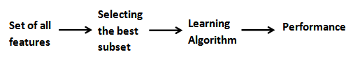
As name suggest, in this method, we filter and take only the subset of the relevant features. The model is built after selecting the features. The filtering is done using correlation matrix and it is most commonly done using Pearson correlation.

Here we will 1st plot the Pearson correlation Heat map and visualize the correlation of independent variables with output variable named MEDV. We will only select features which has correlation of above 0.5 (taking absolute value) with the output variable. The correlation coefficient has values between -1 to 1. We can relate the obtained result as:

A value closer to 0 denotes weaker correlation (exact 0 implying no correlation)

A value closer to 1 denotes stronger positive correlation

A value closer to -1 denotes stronger negative correlation

Filter Method Example:

First we will load boston dataset from sklearn with this command

from sklearn.datasets import load_boston

All independent variables are stored in df, and dependant variable MHDV is stored in y. Here we will see the Heatmap using Pearson correlation as follows:

# Using Pearson Correlation

plt.figure(figsize=(12,10))

cor=df.corr()

sns.heatmap(cor, annot=True, cmap=plt.cm.Reds)

plt.show()

It will show the result in form of heat map as follows:

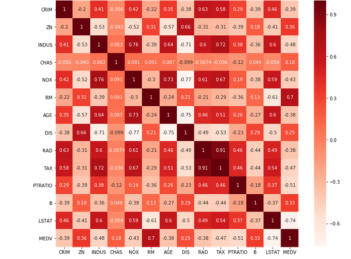
The heat map gives the ides about correlation of all variables including dependant variable. From this we have to choose the set of correlations of features with output (dependant variable) ‘MHDV’ as follows:

# Correlation with output variable MEDV

cor_target=abs(cor[“MEDV”])

From this we will find highly correlated features:

# Selecting highly correlated features

relevant_features=cor_target[cor_target>0.5]

relevant_features

Result:

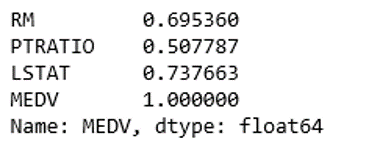
In above step we found fields only which are highly correlated with the output variable MEDV. Those are selected features RM, PTRATIO and LSTAT. We can eliminate other features. Now we have to check the correlation between those fields. Correlation between fields must be less, because as value gets reduced the correlation is strong.

print(df[[“LSTAT”,”PTRATIO”]].corr())

print(df[[“LSTAT”,”RM”]].corr())

print(df[[“RM”,”PTRATIO”]].corr())

According to assumptions of linear regression, the independent variables need to be uncorrelated to each other. If these variables are correlated with each other, then we need to select only one of them and eliminate the rest. So let us check the correlation of selected features with each other.

print(df[[“LSTAT”,”PTRATIO”]].corr())

print(df[[“LSTAT”,”RM”]].corr())

print(df[[“RM”,”PTRATIO”]].corr())

Result:

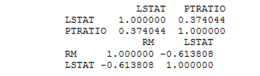
So with this it is recognized that variables RM and LSTAT are highly correlated with each other (-0.613808). Therefore, we would keep only one variable and drop other. We will keep LSTAT since its correlation with MEDV is higher than that of RM. Now we have two selected features with us LASTAT and PTRATIO. And model can be built based on these features.

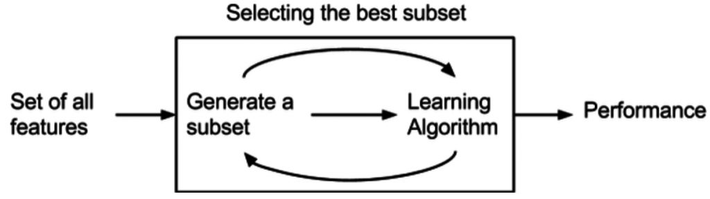
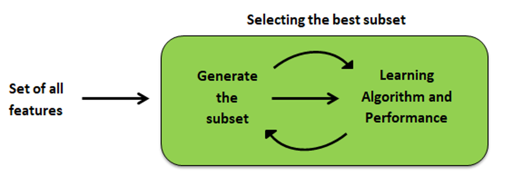
Wrapper Method

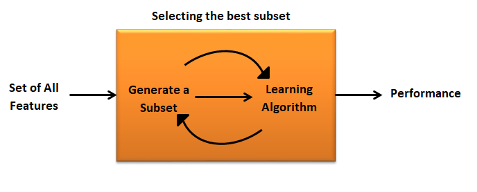
A wrapper method needs one machine learning algorithm and performance of algorithm is used as evaluation criteria. i.e. you feed the features to the selected Machine Learning algorithm and based over the model performance you add or remove the features. It is an iterative and computationally expensive process Still it is more accurate than the filter method.

Forward Selection

It is an iterative method in which initially we have to start with selection of single feature. By observing overall performance we can add the next feature in model. We have to add features till we get best result. By adding features we try to increase performance of model.

Backward Elimination

Here we have to start training model by adding all features and removing one feature in next iteration. It is exactly opposite to forward elimination. The least significant feature will be removed in every iteration to get improved accuracy. Until improvement stops we have to remove features one by one.

Backward Elimination Example

First import the boston data from dataset

from sklearn.datasets import load_boston

import pandas as pd

import numpy as np

import statsmodels.api as sm

from sklearn.model_selection import train_test_split

from sklearn.linear_model import LinearRegression

x=load_boston()

df=pd.DataFrame(x.data, columns = x.feature_names)

df[“MEDV”]=x.target

x=df.drop(“MEDV”,axis=1)

y=df[‘MEDV’]

Till now we decided independent and dependant variables. Now we will apply algorithm and backward elimination process:

# BACKWARD ELIMINATION:

x_1=sm.add_constant(x)

model=sm.OLS(y,x_1).fit()

model.summary()

By checking model summary we can eliminate features having ‘P’ value greater than 0.05.

Otherwise you can write python code as follows:

cols=list(x.columns)

pmax=1

while(len(cols)>0):

p=[]

x_1=x[cols]

x_1=sm.add_constant(x_1)

model=sm.OLS(y,x_1).fit()

p=pd.Series(model.pvalues.values[1:],index=cols)

pmax=max(p)

feature_with_p_max=p.idxmax()

if(pmax>0.05):

cols.remove(feature_with_p_max)

else:

break

selected_features_BE=cols

print(selected_features_BE)

(Here 11 features are selected from 13 features).

Recursive Feature Elimination

It is wrapped method’s algorithm which tries to find the best contributing feature subset. It repetitively creates models and tracks the best or the worst performing feature at each iteration. It designs the next model with the remaining features until all the features are drained. It then ranks the features based on elimination order.

Recursive Feature Elimination Example

We will apply it on same Boston data set. So the process of initialization and storing all variables will be same.

rfe=RFE(model, nof_list[n])

high_score=0

nof=0

score_list=[]

for n in range(len(nof_list)):

X_train, X_test, y_train,y_test=train_test_split(x,y,test_size=0.3,random_state=0)

model=LinearRegression()

rfe=RFE(model, nof_list[n]

x_train_rfe=rfe.fit_transform(X_train,y_train)

x_test_rfe=rfe.transform(X_test)

model.fit(x_train_rfe,y_train)

score=model.score(x_test_rfe,y_test)

score_list.append(score)

if(score>high_score):

high_score=score

nof=nof_list[n]

print(“Optimum number of features: %d” %nof)

print(“Score with %d features: %f” %(nof,high_score))

Embedded Method

Embedded methods carefully extract those features in each iteration, which contribute most for prediction while training the system. Regularization methods are most commonly used embedded methods which penalize a feature with a coefficient threshold.

Embedded methods are combination of filter and wrapper methods. Method is implemented by algorithms that have their integral feature selection methods. Some of the most popular embedded methods like LASSO and RIDGE regression are used to reduce problem of over fitting by penalization.

Lasso regression achieves L1 regularization in which penalty equivalent to absolute value of the magnitude of coefficients is added.

Ridge regression achieves L2 regularization in which penalty equivalent to square of the magnitude of coefficients is added.

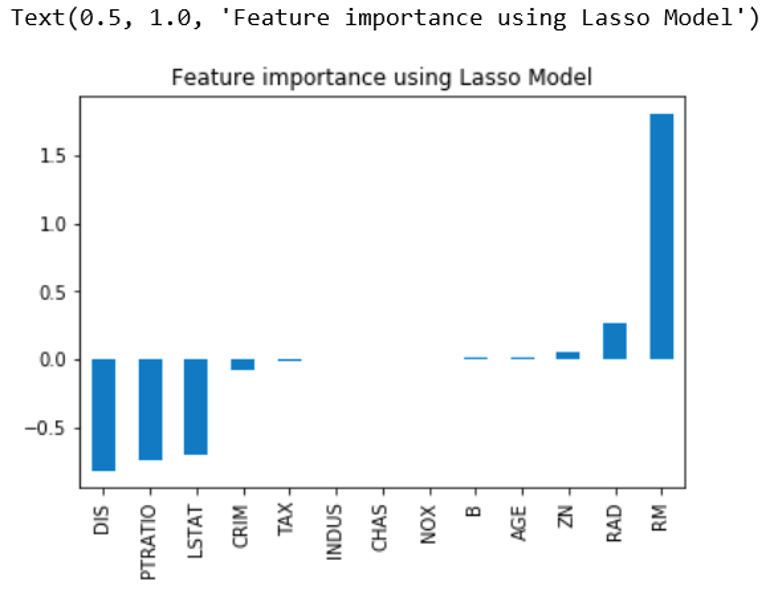
In following example, feature selection is performed using Lasso regularization. If the feature is immaterial, Lasso penalizes its coefficient and make it 0. Hence features with coefficient = 0 are removed and the rest are selected.

LASSO:

As shown in previous example load Boston file

import pandas as pd

import numpy as np

import matplotlib

import matplotlib.pyplot as plt

import seaborn as sns

%matplotlib inline

from sklearn.linear_model import LassoCV, Lasso

reg=LassoCV()

reg.fit(x,y)

print(“Best alpha using built-in LassoCV: %f” % reg.alpha_)

print(“Best score using built-in LassoCV: %f” % reg.score(x,y))

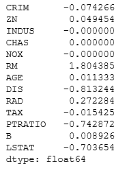
coef=pd.Series(reg.coef_,index=x.columns)

Result

print(“Lasso picked ” + str(sum(coef !=0)) + ” variables and eliminated the others ” +str(sum(coef==0)) + ” varibles”)

Here we are checking how many features selected by printing the statement

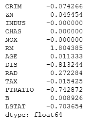
Lasso picked 10 variables and eliminated the others 3 variables.

(Note: The result can be changed according to dataset.)

To get the graphical output we can add following lines in code:

imp_coef=coef.sort_values()

imp_coef.plot(kind=”bar”)

plt.title(“Feature importance using Lasso Model”)

RIDGE:

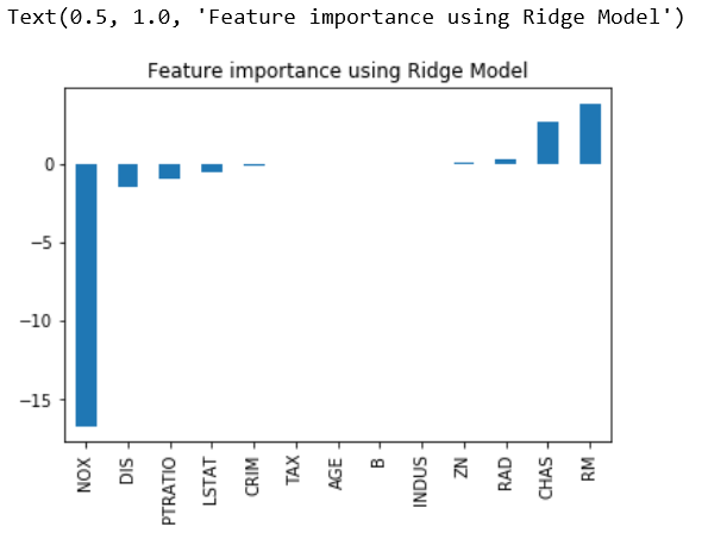
In following example, feature selection is performed using Ridge regularization.

As shown in previous example load boston file

import pandas as pd

import numpy as np

import matplotlib

import matplotlib.pyplot as plt

import seaborn as sns

%matplotlib inline

from sklearn.linear_model import RidgeCV, Ridge

reg=RidgeCV()

reg.fit(x,y)

print(“Best alpha using built-in RidgeCV: %f” % reg.alpha_)

print(“Best score using built-in RidgeCV: %f” % reg.score(x,y))

coef=pd.Series(reg.coef_,index=x.columns)

coef

Result:

print(“Ridge picked ” + str(sum(coef !=0)) + ” variables and eliminated the others ” +str(sum(coef==0)) + ” varibles”)

Here we are checking how many features selected by printing the statement.

Ridge picked 13 variables and eliminated the others 0 variables.

(Note: The result can be changed according to dataset.)

To get the graphical output we can add following lines in code:

imp_coef=coef.sort_values()

imp_coef.plot(kind=”bar”)

plt.title(“Feature importance using Ridge Model”)

We hope you understand the Feature selection tutorial with examples concepts. Get success in your career as a Machine Learning Engineer by being a part of the Prwatech, India’s leading Data Science training institute in Bangalore.