k-Nearest Neighbors Algorithm Tutorial

k-nearest neighbors Algorithm Tutorial, Are you the one who is looking forward to know about knn algorithm introduction in Machine Learning? Or the one who is looking forward to know How KNN algorithm works and benefits of knn or Are you dreaming to become to certified Pro Machine Learning Engineer or Data Scientist, then stop just dreaming, get your Data Science certification course with Machine Learning from India’s Leading Data Science training institute.

Knn is part of supervised learning which will be used in many applications such as data mining, image processing and many more. It is simple and one of the most important Machine learning algorithms. In this blog, we will learn knn algorithm introduction, knn implementation in python and benefits of knn. Do you want to know How KNN algorithm works, So follow the below mentioned k-nearest neighbors algorithm tutorial from Prwatech and take advanced Data Science training with Machine Learning like a pro from today itself under 10+ Years of hands-on experienced Professionals.

knn Algorithm Introduction

K nearest Neighbor (KNN) is a popular supervised machine learning algorithm that is used widely. Its popularity stems from its comfort of use, and its clearly reasonable results. The ‘K’ in KNN indicates the number of nearest neighbors, which are used to classify or predict outputs in a data set. The classification or prediction of every new data point is based on a specific distance calculated from nearest neighbors and their weighted averages.

If there is very little prior knowledge about the distribution of data points, KNN emerges as the best algorithm for analysis. When dealing with labeled datasets, KNN aids in discovering the relationship between each observation in the training data. This relationship, often referred to as resemblance, is quantified using a distance metric between data points. Various methods exist to compute these intervals, including Euclidean, Manhattan, Chebyshev, and Hamming distance.

KNN operates as a non-parametric algorithm, making no explicit assumptions about the functional form of the relationship. Instead, it directly operates on training instances without applying any predefined model. Although KNN can be utilized to tackle prediction problems in both classification and regression, its predominant usage lies in classification prediction within the industry.

How KNN algorithm works?

As mentioned above KNN basically works on the relationship of resemblance by means of calculating distance of data point from others.

Let’s take an example.

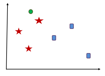
Let’s consider a set of some data points is given which includes red stars and blue squares. Now we have to categorize a new data point which is indicated with green circle. For applying KNN, first we have to decide value of K. Let’s consider value of K be 3. Now based on K=3 we have to find 3 neighbors which are nearest to this green circle.

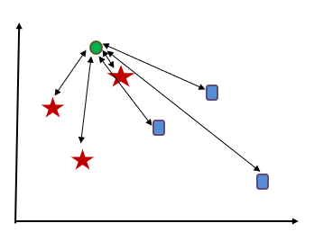
In this example the green circle has to find its nearest neighbors. And as we can see all the red stars are nearest to the circle compared to blue squares. So, the new data point i.e. green circle will be classified as ‘red star’.

To get best possible fit for the data set, it is important to select the appropriate value of ‘K’ i.e. number of nearest neighbors. If K value is small, the region of prediction is restricted and it makes the classifier less sensitive the overall distribution. K should be most common class value in case of classification and it should be mean output variable in case of regression.

Methods of calculating distance between data points:

To find the distance of target data point means to measure the interval between new data point and each data point present around it.  To calculate this the most commonly used methods are: Euclidian, Manhattan and Hamming distance.

Euclidian Distance:

It is the square root of the sum of the squared differences between a new point and an existing point. Let’s take new point as x and existing point y.

Manhattan Distance:

It is the distance between real vectors using the sum of their absolute difference.

Hamming Distance:

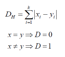
Hamming distance is helpful in case of categorical variables. If the x value and y value are same, the distance will be zero. Otherwise distance is:

Here distance is indicated with ‘D’.

How to decide K value?

The most important step in KNN is to determine the optimal value of K. The optimal value of k decreases effect of the noise on the classification. For this a technique called ‘Elbow method’ helps to select the optimal K value.

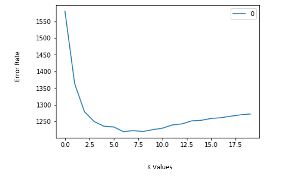
Let’s say we are applying K with different values to same dataset. Initially we have to observe the error rate changing with K values. Let’s say we applied KNN on a data set and we got a curve of error rate Vs. K values as follows:

Here we can observe that initially error rate is decreasing up to nearly 6. After that it starts increasing. So, the value of K should be 6 i.e. it is optimum value of K for this model. This curve is called because it has a shape like an elbow and is usually used to regulate the k value. This is called Elbow method.

knn implementation in python

In the following example we will consider k=3, hence, we will take 3 nearest points to new or target point.

Importing Library

Importing dataset

df= pd.read_csv(“ Your File Path”)

(We will consider that necessary cleaning part is done)

Divide the dataset into independent and dependent parts.

X = data.iloc[:,0:20]  #independent columns

y = data.iloc[:,-1] # target column

Split the dataset into two parts for training and testing.

from sklearn.model_selection import train_test_split

X_train, X_test, y_train, y_test = train_test_split(X, y, random_state = 10, test_size = 0.33)

Preprocessing – Scaling the features

from sklearn.preprocessing import MinMaxScaler

scaler = MinMaxScaler(feature_range=(0, 1))

x_train_scaled = scaler.fit_transform(x_train)

x_train = pd.DataFrame(x_train_scaled)

x_test_scaled = scaler.fit_transform(x_test)

x_test = pd.DataFrame(x_test_scaled)

Visualize the error rate for different k values

#import required packages

%matplotlib inline

rmse_val = []

#to store rmse values for different k

for K in range(20):

K = K+1

model = neighbors.KNeighborsRegressor(n_neighbors = K)

model.fit(x_train, y_train)           #fit the model

pred=model.predict(x_test)          #make prediction on test set

error = sqrt(mean_squared_error(y_test,pred))

#calculate rmse

rmse_val.append(error) #store rmse values

print(‘RMSE value for : ‘ , K , ‘is:’, error)

#plotting the rmse values against k values

curve = pd.DataFrame(rmse_val)     #elbow curve

curve.plot()

Implementing GridsearchCV

Plotting the elbow curve every time to determine K, is be a cumbersome and tedious process. You can simply use gridsearch to find the best value.

from sklearn.model_selection import GridSearchCV

params = {‘n_neighbors’:[2,3,4,5,6,7,8,9]}

knn = neighbors.KNeighborsRegressor()

model = GridSearchCV(knn, params, cv=5)

model.fit(x_train,y_train)

model.best_params_

Benefits of knn:

The algorithm is useful in searching for similar documents. This algorithm can be used to find all the e-mails, briefs, contracts, etc. relevant to given problem statements. Recommendation systems prefer this algorithm to recommend customer different products based on past purchasing history. Also, it is used as a benchmark for more complex classifiers such as Artificial Neural Networks (ANN).

We hope you understand k-nearest neighbors algorithm tutorial.Get success in your career as a Data Scientist by being a part of the Prwatech, India’s leading Data Science training institute in Bangalore.