Binomial Probability Distribution
Binomial Distribution: Conditions, Formula and Worked Examples
A call centre agent connects with a customer on 8 out of every 10 calls, on average. Tomorrow she makes 10 calls. How likely is it that she connects exactly 7 times? Or at least 7 times? Questions like these, with a fixed number of tries and a yes or no result each time, are the home ground of the binomial distribution.
It is one of the most used distributions in practice. Quality checks, click through rates, survey responses, medical trials and A and B tests all count successes in a fixed number of tries. It also builds directly on the Bernoulli trial, the simplest random experiment, and leads to the normal distribution and to hypothesis tests.
This tutorial explains the four conditions that make a situation binomial, the formula, how to work through an example step by step, the mean and variance, and how to get the answers in Excel and Python. You should know what a random variable is. If not, start with our random variable tutorial.
What is a Binomial Probability Distribution?
A binomial distribution gives the probability of getting exactly k successes in n independent trials, when each trial has only two outcomes and the same chance of success. The word binomial means two names, here success and failure.
The two outcomes are just labels. Success means the outcome you are counting, whether it is good or bad. In a quality check, a defective item can be the success.
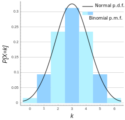
Bernoulli Trial: The Building Block
A Bernoulli trial is a single experiment with two outcomes, such as one coin toss, one call, or one product tested. The chance of success is p, and the chance of failure is 1 minus p. A binomial distribution is what you get from n such trials. With n = 1 it is the Bernoulli distribution itself. For p = 0.3, it gives 0.7 for failure and 0.3 for success.
The Four Conditions
Check all four before you use the binomial formula.
- A fixed number of trials, called n. You decide it in advance.
- Two outcomes in each trial, success or failure.
- The same probability of success, p, in every trial.
- Independent trials. The result of one trial does not change the chance in the next.
A Quick Test: Is It Binomial?
| Situation | Binomial? | Reason |
|---|---|---|
| Toss a coin 20 times, count the heads | Yes | All four conditions hold |
| Make 10 calls, count the connected ones, with p = 0.8 for each | Yes | Fixed n, two outcomes, same p |
| Draw 3 cards from a deck without putting them back, count the hearts | No | The chance changes after each draw, so the trials are not independent |
| Toss a coin until the first head | No | The number of trials is not fixed |
Drawing without replacement from a very large population is close enough to independent, so the binomial is often used there as an approximation. For a small group, it is not accurate.
Binomial Probability Distribution Formula
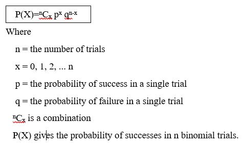
- n is the number of trials.
- k is the number of successes you want.
- p is the probability of success in one trial.
- (n choose k) is the number of ways to pick which k of the n trials are the successes. It equals n factorial divided by (k factorial times (n minus k) factorial).
The formula has two parts. The first, n choose k, counts the different orders in which the successes can happen. The second, p to the power k times (1 minus p) to the power (n minus k), is the probability of any one such order.
Binomial Probability Distribution Example
Question: the chance of a call connecting is 0.8. Find the probability of exactly 7 connected calls in 10 attempts.
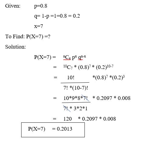
- Identify the values: n = 10, k = 7, p = 0.8, and 1 minus p = 0.2.
- Count the ways. 10 choose 7 = 120.
- Find the probability of one order. 0.8 to the power 7 times 0.2 to the power 3.
- Multiply: 120 times 0.8 to the power 7 times 0.2 to the power 3 = 0.2013.
The probability of exactly 7 connected calls is 0.2013, or about 20.1 percent. The live page does not state this answer in text.
The Whole Distribution
| Connected calls (k) | P(X = k) |
|---|---|
| 0 to 4 together | 0.0064 |
| 5 | 0.0264 |
| 6 | 0.0881 |
| 7 | 0.2013 |
| 8 | 0.3020 |
| 9 | 0.2684 |
| 10 | 0.1074 |
| Total | 1.0000 |
Exactly 8 connections is the most likely result, which makes sense for an 80 percent rate. Exactly 7 comes next.
At Most, At Least and Cumulative Probabilities
Often you need more than one value of k. Add the individual probabilities.
| Question | Answer |
|---|---|
| P(X is at most 7) | 0.3222, which is the sum of k = 0 to 7 |
| P(X is at least 7) | 0.8791, which is 0.2013 plus 0.3020 plus 0.2684 plus 0.1074 |
| P(X = 10), all calls connect | 0.1074 |
A useful trick: at least 7 equals 1 minus the probability of at most 6, so you can use whichever side has fewer terms.
Mean, Variance and Standard Deviation
| Measure | Formula | For n = 10, p = 0.8 |
|---|---|---|
| Mean | n times p | 8 |
| Variance | n times p times (1 minus p) | 1.6 |
| Standard deviation | The square root of the variance | 1.265 |
So the agent connects with 8 customers on average, with a typical swing of about 1.3 calls either way.
Coin Toss Example: What Really Happens in 20 Tosses
The live page suggests that after 20 tosses, a tail becomes very close to certain. Here are the exact numbers for a fair coin tossed 20 times.
- The expected number of tails is 20 times 0.5 = 10.
- The probability of at least one tail is 1 minus 0.5 to the power 20 = 0.999999.
- The probability of exactly 10 heads is only 0.1762, so an even split is not guaranteed.
- The probability of 8 to 12 heads is 0.7368.
The point to remember: results near the expected value are likely, but one exact value usually has a modest probability.
A Quality Control Example
Suppose 10 percent of items from a machine are defective. You pick 5 items. This is my own example, and it assumes the items are independent. The probability of no defects is 0.9 to the power 5 = 0.5905. The probability of at least one defect is 1 minus 0.5905 = 0.4095. So even with a 10 percent defect rate, about two in five samples of 5 will contain a defect.
Calculate It in Excel, a Calculator and Python
The live page mentions TI 83 and TI 89 calculators. Most readers use Excel or Python today. In Excel, BINOM.DIST takes the number of successes, the number of trials, the probability and a true or false for cumulative. In Python, SciPy does it in one line. I ran the code below, and the output is real.
A simulation of one million sets of 10 calls gave P(X = 7) = 0.2019, close to the exact 0.2013.
Common Mistakes to Avoid
| Mistake | Fix |
|---|---|
| Using the formula when trials are not independent | Check the four conditions first |
| Forgetting the n choose k part | Without it you only get the probability of one order |
| Mixing up p and 1 minus p | p is the success you are counting |
| Using exactly when the question says at least | Add the probabilities or use the opposite event |
| Using a changing probability | p must be the same in every trial |
| Rounding too early | Keep full decimals until the last step |
Practice Questions
- A fair coin is tossed 5 times. Find the probability of exactly 2 heads.
- 5 items are picked from a machine with a 10 percent defect rate. Find the probability of at least one defect.
- For n = 100 and p = 0.3, find the mean, variance and standard deviation.
- Three cards are drawn from a deck without replacement. Why is the number of hearts not binomial?
Answers: 1) 10 times 0.5 to the power 5 = 0.3125. 2) 1 minus 0.9 to the power 5 = 0.4095. 3) Mean 30, variance 21, standard deviation 4.58. 4) The chance of a heart changes after each draw, so the trials are not independent. These are my own calculations, so please recheck them before publishing.
The binomial distribution rewards one habit above all: check the four conditions before you calculate. Once they hold, the formula is short, and Excel or Python can do the arithmetic for you. Try the practice questions, and then explore the normal and Poisson distributions that grow out of it.
