Standard Deviation Tutorial
Standard Deviation: Definition, Formula and Worked Examples
Two machines fill 50 gram packets. Over a day, both average exactly 50 grams. One makes packets that all weigh between 49.8 and 50.2. The other makes packets from 46.5 to 53.5. Same average, very different machines. The average cannot tell them apart, and standard deviation can.
Standard deviation is the number that says how far values typically sit from their mean. It is one of the most used ideas in data science, in quality control, in finance, and in every statistics course. You will see it in z scores, in confidence intervals, in feature scaling and in outlier detection.
This tutorial explains what it means, how to calculate it by hand on two examples, the difference between the population and the sample version, the 68 95 99.7 rule, and how to get it in Python. If you are new, read our measures of central tendency and sample variance tutorials first.
Standard Deviation Definition in Statistics
Standard deviation measures how spread out the values of a dataset are around their mean. A low value means the data sits close to the mean. A high value means it is scattered. The higher the dispersion, the greater the standard deviation.
It is the square root of the variance. Variance is in squared units, such as square millimetres, which is hard to picture. Taking the square root brings you back to the original unit, so a standard deviation of 147 mm can be read as 147 mm.
Example of Standard Deviation: Heights of Dogs
You measure the heights, at the shoulder, of five dogs. They are 600, 470, 170, 430 and 300 millimetres.
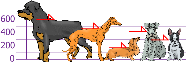
Let us plot these on a chart, and then find the mean.
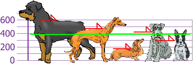
The mean is (600 plus 470 plus 170 plus 430 plus 300) divided by 5 = 1970 divided by 5 = 394 mm. Now find how far each dog is from the mean.
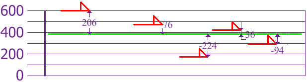
| Height | Minus the mean (394) | Squared |
|---|---|---|
| 600 | 206 | 42,436 |
| 470 | 76 | 5,776 |
| 170 | minus 224 | 50,176 |
| 430 | 36 | 1,296 |
| 300 | minus 94 | 8,836 |
| Total | 0 | 108,520 |
- Variance = 108,520 divided by 5 = 21,704 (square millimetres)
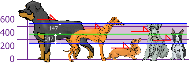
- Standard deviation = the square root of 21,704 = 147.32, so about 147 mm
Now you have a yardstick. The range of one standard deviation around the mean runs from 394 minus 147 to 394 plus 147, which is about 247 mm to 541 mm. Dogs of 470, 430 and 300 mm fall inside the range, so they count as normal. The dogs of 600 mm and 170 mm fall outside it, so they are extra tall and extra short.
Why Use Standard Deviation?
- To compare spread. Two datasets with the same mean can behave very differently, as the machine example shows.
- To judge what is normal. A value within one or two standard deviations of the mean is usual. A value far outside it deserves a look.
- To measure consistency and risk. A low value for a machine means steady output. A high value for an investment means bigger swings.
- As an input to other tools. Z scores, confidence intervals, hypothesis tests and feature scaling all use it.
How to Calculate Standard Deviation
- Find the mean of the data.
- Subtract the mean from every value. These are the deviations.
- Square each deviation.
- Add up the squared deviations.
- Divide by N for a population, or by N minus 1 for a sample. This gives the variance.
- Take the square root of the variance.
Standard Deviation Formula
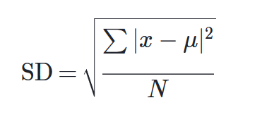
| Feature | Population | Sample |
|---|---|---|
| Symbol | sigma | s |
| Mean symbol | mu | x bar |
| Divide the sum of squares by | N | N minus 1 |
| Use when | You have every member of the group | You have a part of the group and want to estimate the whole |
In real work you almost always have a sample, so you use N minus 1. The reason is explained in our sample variance tutorial. The live version of this page divides by N, which is the population method. That is correct if the dogs are the whole group you care about, and it is not correct if five dogs stand for all dogs. For the dogs, the sample standard deviation is 164.71 mm, against 147.32 mm for the population version.
Example 2: Ten Numbers
The data is 4, 2, 3, 5, 2, 2, 6, 1, 4, 2. The sum is 31, and there are 10 values, so the mean is 3.1.
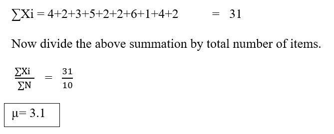
Subtract the mean, 3.1, from every item and square the result.
| Value | Value minus 3.1 | Squared |
|---|---|---|
| 4 | 0.9 | 0.81 |
| 2 | minus 1.1 | 1.21 |
| 3 | minus 0.1 | 0.01 |
| 5 | 1.9 | 3.61 |
| 2 | minus 1.1 | 1.21 |
| 2 | minus 1.1 | 1.21 |
| 6 | 2.9 | 8.41 |
| 1 | minus 2.1 | 4.41 |
| 4 | 0.9 | 0.81 |
| 2 | minus 1.1 | 1.21 |
| Total | 0 | 22.9 |
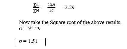
The live page stops here. Here is the finish.
| Measure | Population (divide by 10) | Sample (divide by 9) |
|---|---|---|
| Variance | 2.29 | 2.54 |
| Standard deviation | 1.51 | 1.60 |
What Does the Number Tell You?
A standard deviation has no good or bad value by itself. It must be read against the mean and the context. A standard deviation of 5 mm is huge for a bolt and tiny for the height of a building.
The 68 95 99.7 Rule
If the data follows a bell shaped, normal pattern, about 68 percent of values fall within one standard deviation of the mean, about 95 percent within two, and about 99.7 percent within three. I checked this with a simulation of one million normal values with a mean of 100 and a standard deviation of 15.
| Range around the mean | Share of values |
|---|---|
| Within 1 standard deviation | 68.3 percent |
| Within 2 standard deviations | 95.4 percent |
| Within 3 standard deviations | 99.7 percent |
Use the rule with care. It holds for normal data. For skewed data, such as incomes, the shares are different.
Z Score
A z score says how many standard deviations a value is from the mean. It equals (value minus mean) divided by standard deviation. The 600 mm dog has a z score of (600 minus 394) divided by 147.32 = 1.40. It is 1.4 standard deviations above the mean. A common rule of thumb flags values with a z score beyond 3 as outliers, but it is a guide, not a law.
Comparing Two Machines
Back to the packets. Five packets from each machine, in grams:
| Machine | Weights | Mean | Sample SD |
|---|---|---|---|
| A | 49.8, 50.1, 50.0, 49.9, 50.2 | 50.0 | 0.16 |
| B | 47.0, 53.5, 50.2, 46.5, 52.8 | 50.0 | 3.22 |
Both average 50.0 grams. Machine A has a standard deviation of 0.16 g, and machine B has 3.22 g. Machine B is about 20 times more spread out, and a weight check with a tight limit would reject many of its packets. This is my own example. Only five readings each, so treat it as an illustration, not a quality study.
Calculate Standard Deviation in Python
Remember the defaults. The statistics module has two functions, stdev for samples and pstdev for populations. NumPy divides by N by default. pandas divides by N minus 1 by default. I ran the code below, and the output is real.
| Library | Sample SD | Population SD |
|---|---|---|
| statistics | stdev() | pstdev() |
| NumPy | np.std(x, ddof=1) | np.std(x), the default |
| pandas | Series.std(), the default | Series.std(ddof=0) |
Common Mistakes to Avoid
| Mistake | Fix |
|---|---|
| Using the population formula for a sample | Divide by N minus 1 and use s |
| Forgetting the square root, so you report the variance | Take the square root as the last step |
| Subtracting the sum instead of the mean | Subtract the mean |
| Using np.std and assuming it is the sample version | Set ddof=1 |
| Applying the 68 95 99.7 rule to skewed data | Check the shape of the data first |
| Calling a standard deviation large or small with no context | Compare with the mean, or use another dataset |
Practice Questions
- Find the population standard deviation of 2, 4, 4, 4, 5, 5, 7, 9.
- Find the sample standard deviation of 10, 12, 14.
- A dataset has a mean of 60 and a standard deviation of 8. What is the z score of 76?
Answers: 1) Mean 5, squared deviations 9, 1, 1, 1, 0, 0, 4, 16 add to 32, variance 4, standard deviation 2. 2) Mean 12, squares 4, 0, 4 add to 8, divided by 2 gives 4, standard deviation 2. 3) (76 minus 60) divided by 8 = 2. These are my own calculations, so please recheck them before publishing.
Standard deviation turns the question how spread out is my data into a single number you can compare and act on. Calculate a few by hand to build the feel, check whether you need the sample or population version, and then let Python do the work.
