Mean and variance of Bernoulli distribution
Mean and Variance of the Bernoulli Distribution: Formula and Examples
A machine makes a bolt. It is either good or defective. A customer opens an email. They either click or do not click. A match ends. A team either wins or loses. In each case there is one try and two possible results. The Bernoulli distribution is the simplest model for this.
It looks too simple to matter, yet it sits underneath much of data science. Classification models, click rate tests, quality checks and the binomial distribution are all built from Bernoulli trials. Two numbers describe it fully: the mean and the variance, and both come from a single value, p.
This tutorial explains what a Bernoulli distribution is, derives the mean and variance in a few lines, works through three examples with all the numbers, shows the link to the binomial distribution, and finishes with Python code and practice questions.
What is the Bernoulli Distribution?
The Bernoulli distribution is a discrete probability distribution for a single trial that has only two outcomes. One outcome is called a success and the other a failure. A success is coded as 1 and a failure as 0.
- The probability of success is p.
- The probability of failure is q = 1 minus p.
A coin toss with heads as success has p = 0.5. For a coin, failure means tails, so the probability of failure is 1 minus 0.5 = 0.5. The live page says the probability of failure is 1 minus the probability of heads, which is true, but it never says that this is tails.
Suppose success has a probability of 0.7. Then failure has 0.3. The distribution is just two bars: a bar of height 0.3 at 0, and a bar of height 0.7 at 1.
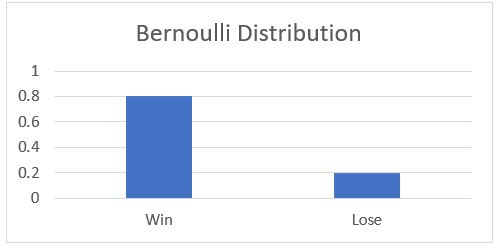
| Outcome | Value of X | Probability |
|---|---|---|
| Failure | 0 | 1 minus p |
| Success | 1 | p |
A Bernoulli trial is a special case of the binomial distribution with n = 1, which means one trial. Bernoulli is the building block. Binomial counts the successes in many trials.
Conditions for a Bernoulli trial: there is one trial, only two outcomes, and a fixed probability of success p.
Mean and Variance of the Bernoulli Distribution Formula
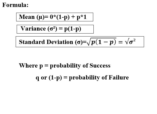
| Measure | Formula |
|---|---|
| Mean (expected value) | E(X) = p |
| Variance | Var(X) = p times (1 minus p) = p times q |
| Standard deviation | The square root of p times (1 minus p) |
Why These Formulas are True?
The mean is each value times its probability, added up:
For the variance, first find the mean of X squared. Since X is 0 or 1, X squared is the same as X, so E(X squared) = p. Then:
That is all. The mean tells you the long run share of successes, and the variance tells you how unsure each trial is.
When is the Variance Biggest?
| p | Variance p times (1 minus p) | Reading |
|---|---|---|
| 0.1 | 0.09 | Failure is very likely, so little surprise |
| 0.3 | 0.21 | |
| 0.5 | 0.25 | The biggest, a fair coin |
| 0.7 | 0.21 | |
| 0.9 | 0.09 | Success is very likely, so little surprise |
The variance is largest at p = 0.5, where the outcome is hardest to guess. It falls toward 0 as p moves toward 0 or 1, when the outcome is nearly certain. The maximum is 0.25.
Mean and Variance of the Bernoulli Distribution Example
Example 1: The Page Example, Reframed
The live page asks for the mean, variance and standard deviation when the probability of India winning the 2019 cricket World Cup is 80 percent. That tournament is over, so I treat it as a team that has an 80 percent chance of winning one match. The number is made up.
- p = 0.8, and q = 0.2.
- Mean = p = 0.8.
- Variance = 0.8 times 0.2 = 0.16.
- Standard deviation = the square root of 0.16 = 0.4.
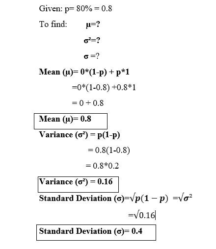
Meaning: across many such matches, the team wins 80 percent of the time on average. The standard deviation of 0.4 is large next to the mean of 0.8, which is normal for a 0 or 1 outcome.
Example 2: A Success Probability of 0.7
The page’s 0.7 and 0.3 picture: p = 0.7.
- Mean = 0.7.
- Variance = 0.7 times 0.3 = 0.21.
- Standard deviation = the square root of 0.21 = 0.4583.
Example 3: A Defect Rate (Quality Control)
A line makes bolts, and 5 percent are defective. Let success mean a defective bolt, so p = 0.05. The numbers are made up.
- Mean = 0.05.
- Variance = 0.05 times 0.95 = 0.0475.
- Standard deviation = 0.2179.
Meaning: each bolt has a 5 percent chance of being defective. The variance is small, because the outcome is mostly the same: not defective.
Bernoulli vs Binomial Distribution
| Point | Bernoulli | Binomial |
|---|---|---|
| Trials | One | n trials |
| What it counts | Success or failure, 1 or 0 | Number of successes, 0 to n |
| Mean | p | n times p |
| Variance | p times (1 minus p) | n times p times (1 minus p) |
| Link | A binomial with n = 1 | A sum of n independent Bernoulli trials |
Add up n independent Bernoulli trials and the means add to n times p, and the variances add to n times p times (1 minus p). With n = 10 and p = 0.7, the mean is 7 and the variance is 2.1. The live page uses the word binomial in its intro and closing lines where it means Bernoulli. They are close relatives but not the same.
Where the Bernoulli Distribution is Used?
- Classification models. Each prediction is a Bernoulli outcome, such as fraud or not fraud.
- A and B tests. Each visitor either converts or does not.
- Quality control. Each item is defective or not.
- Logistic regression. It models the p of a Bernoulli outcome.
Bernoulli Distribution in Python
I ran the code below, and the output is real.
The simulated mean of 0.6997 and variance of 0.2101 are close to the theory values of 0.7 and 0.21.
Common Mistakes to Avoid
| Mistake | Fix |
|---|---|
| Calling Bernoulli and binomial the same thing | Bernoulli is one trial. Binomial is n trials |
| Forgetting that the variance is p times (1 minus p) | Not p alone, and not p squared |
| Using the mean as a possible outcome | A single trial gives 0 or 1, never 0.7 |
| Mixing up success and failure | Define success clearly before you calculate |
| Assuming p changes between trials | A Bernoulli trial has a fixed p |
| Using it for more than two outcomes | Use a categorical or multinomial distribution |
| Using the sample variance formula by habit | The theory variance here is p times (1 minus p) |
Practice Questions
- p = 0.6. Find the mean, variance and standard deviation.
- For what p is the variance of a Bernoulli trial largest, and what is it?
- A trial has a success probability of 0.2. What is the probability of failure?
- A binomial has n = 20 and p = 0.3. Find its mean and variance.
Answers: 1) Mean 0.6, variance 0.6 times 0.4 = 0.24, standard deviation 0.4899. 2) p = 0.5, variance 0.25. 3) 0.8. 4) Mean 20 times 0.3 = 6, variance 20 times 0.3 times 0.7 = 4.2. These are my own answers, so please recheck them before publishing.
The Bernoulli distribution takes one number, p, and gives you everything: the mean is p and the variance is p times (1 minus p). Learn it well, and the binomial distribution, logistic regression and click rate tests all become easier to follow.
