Uniform Distribution tutorial
Uniform Distribution: Definition, Formula and Examples
You roll a fair die. Each face from 1 to 6 has exactly the same chance. Now think of a bus that comes at some random moment in a 15 minute window. Any moment is as likely as any other. These two situations look different, but they share one idea: no outcome is favoured. That idea is the uniform distribution.
It is the simplest probability distribution, and also one of the most useful. Random number generators produce uniform values, simulations start from them, and they are a fair way to say we know the range but nothing else. Understanding it also makes the harder distributions, such as the normal, easier to follow.
In this tutorial you will learn what a uniform distribution is, the difference between the discrete and continuous kinds, the formulas for probability, mean, variance and standard deviation, a worked example that corrects an error that is common online, real examples, and Python code to check it all. If you are new to the topic, read our random variable tutorial first.
What is a Uniform Distribution?
A uniform distribution is a probability distribution in which every outcome in the range is equally likely. The word is exact: not nearly equal, but equal. When you draw its graph, you get a flat, rectangular shape, so it is also called a rectangular distribution.
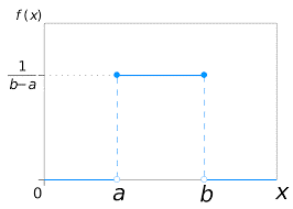
Types of Uniform Distribution
| Feature | Discrete uniform | Continuous uniform |
|---|---|---|
| Values | A countable set, such as 1 to 6 | Any value between a and b |
| Example | A fair die, a lottery number | Waiting time for a bus that comes at a random moment |
| Probability of one value | The same for every value, 1 divided by n | Zero for any single exact value |
| Described by | Probability mass function | Probability density function |
| Graph | Bars of equal height | A flat line, a rectangle |
Discrete Uniform Distribution
A discrete uniform variable takes a fixed number of separate values, and each has the same probability. If there are n values, each has probability 1 divided by n.
Example: a fair die has n = 6. For x = 1, 2, 3, 4, 5 or 6, P(X = x) = 1 divided by 6, which is about 0.1667. The live page says the uniform distribution variable is 1 over 6. To be exact, it is the probability of each outcome that equals 1 over 6. The variable itself is the number shown.
For the die, the mean is 3.5. The variance is (n squared minus 1) divided by 12 = 35 divided by 12 = 2.9167, and the standard deviation is 1.7078.
Continuous Uniform Distribution
A continuous uniform variable can take any value between a lower limit a and an upper limit b. The density is the same everywhere inside the range, and zero outside.

The height of the rectangle is 1 divided by (b minus a), and its width is (b minus a), so the total area is 1, as any probability distribution needs. For a range from 1 to 4, the width is 3, and the height is 1 divided by 3, about 0.3333.
To find the probability of a range, multiply the height by the width of the range you want. For example, P(2 < X < 3) = 1 divided by 3 = 0.3333. The probability of any one exact value is zero, because it has no width.
How to Calculate the Uniform Random Variable: Mean, Variance and Standard Deviation
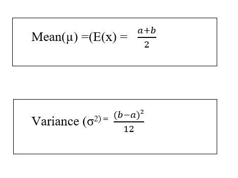
| Measure | Continuous, between a and b | Discrete, n values |
|---|---|---|
| Mean | (a plus b) divided by 2 | (first plus last) divided by 2 |
| Variance | (b minus a) squared divided by 12 | (n squared minus 1) divided by 12 |
| Standard deviation | (b minus a) divided by the square root of 12 | The square root of the variance |
Uniform Distribution Example: Standard Deviation Between 1 and 4
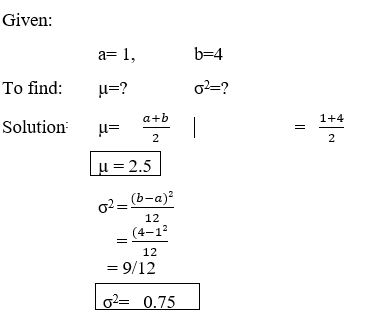
Question: a variable is uniformly distributed between 1 and 4. Find its mean, variance and standard deviation.
- The limits are a = 1 and b = 4, so b minus a = 3.
- Mean = (1 plus 4) divided by 2 = 2.5.
- Variance = 3 squared divided by 12 = 9 divided by 12 = 0.75.
- Standard deviation = the square root of 0.75 = 0.866.
The live page gives 0.75 as the standard deviation. That is the variance. The standard deviation is the square root of it, 0.866. I checked this with SciPy, and with a simulation of one million random values, which gave a mean of 2.5 and a standard deviation of 0.866.
A Real Example: Waiting for a Bus
Suppose a bus arrives at some random time within a 15 minute window, and you reach the stop at a random moment inside it. Your wait is uniform between 0 and 15 minutes. This is my own example, and it assumes that the arrival moment is truly random.
| Question | Answer |
|---|---|
| Average wait | 7.5 minutes |
| Standard deviation of the wait | 4.33 minutes |
| Chance of waiting more than 10 minutes | 0.3333, which is 5 divided by 15 |
Other places you will meet the uniform distribution: random number generators, which produce numbers between 0 and 1, rounding errors, and the first step of simulations, where uniform random numbers are turned into other distributions.
Check It in Python
I ran the code below, and the output is real. In SciPy, uniform takes a starting point, called loc, and a width, called scale, so the range from 1 to 4 is loc = 1 and scale = 3.
Rolling a die 600,000 times in the same way gave a share of 0.166 to 0.167 for every face, close to the exact 0.1667.
Uniform Distribution and Normal Distribution
| Feature | Uniform | Normal |
|---|---|---|
| Shape | Flat, a rectangle | Bell shaped |
| Which values are likelier | None, all are equal | Values near the mean |
| Tails | Stop sharply at a and b | Stretch out without a hard end |
| Defined by | The limits a and b | The mean and the standard deviation |
| Use when | You know the range and nothing else | Data clusters around an average |
Common Mistakes
| Mistake | Fix |
|---|---|
| Reporting the variance as the standard deviation | Take the square root of the variance |
| Saying the outcomes are nearly equal | They are exactly equally likely |
| Using the discrete formula for a continuous range | Use (b minus a) squared divided by 12 for continuous data |
| Asking for P(X = one exact value) in a continuous case | Ask for a range |
| Forgetting that SciPy uses loc and scale, not a and b | Set scale to b minus a |
| Treating any random sample as uniform | Check the shape of the data first |
Practice Questions
- X is uniform between 0 and 10. Find the mean, the variance and the standard deviation.
- For the same X, find P(2 < X < 5).
- A fair ten sided die has faces 1 to 10. Find its variance.
Answers: 1) Mean 5, variance 100 divided by 12 = 8.33, standard deviation 2.89. 2) The width is 3 and the density is 1 divided by 10, so the probability is 0.3. 3) (10 squared minus 1) divided by 12 = 99 divided by 12 = 8.25. These are my own calculations, so please recheck them before publishing.
The uniform distribution is easy, so it is a good place to build habits: write the range, find the density, multiply by the width, and take the square root for the standard deviation. Check your answer with a quick simulation. Then move on to the normal distribution with a clear baseline.
