Mean squared error of regression line
Mean Squared Error of a Regression Line: Formula and Worked Example
You build a model that predicts a person’s weight from their height. It gives an answer for every person, and every answer is a little wrong. How wrong is the model overall? You need one number that sums up all the misses. The most common choice is the mean squared error, or MSE.
MSE sits behind a great deal of data science. It is the quantity that linear regression minimises when it fits a line, it is a standard way to compare models, and its square root, RMSE, is reported in almost every forecasting project. If you understand MSE, you understand how a regression line is chosen.
This tutorial explains what a regression line is, how to find it, how to calculate the mean squared error step by step on a small dataset, how to judge whether a given MSE is good, how it differs from RMSE and MAE, and how to check it in Python. Read our regression analysis tutorial first if the basics are new to you.
What is a Regression Line?
Regression studies the link between a dependent variable, written Y, and one or more independent variables, written X. The regression line is the straight line that best describes how Y changes with X. It is used to explain the relationship and to predict Y for a new X.
Regression is a general statistical method. It is used in finance, but also in medicine, engineering, marketing, agriculture and many other areas.
Why do We Use Regression?
- To predict. Estimate a weight from a height, sales from advertising, or demand from price.
- To explain. Find out how much Y changes when X changes by one unit.
- To compare factors. With several inputs, see which ones matter more.
How to Calculate the Regression Line
There are two basic types. Linear regression uses one independent variable, and multiple regression uses two or more. Curved relationships need non linear methods, which we do not cover here.
- a is the intercept, the value of Y when X is 0.
- b is the slope, how much Y changes when X rises by 1.
- u is the error term, the part of Y that the line cannot explain. Its sample version, the gap between an actual and a predicted value, is called a residual.
The line is found by the method of least squares. It picks the a and b that make the total of the squared errors as small as possible. For one input, the formulas are:
Mean Squared Error of Regression
The error of one prediction is the actual value minus the predicted value. To measure the whole line, you square each error, add up the squares, and divide by the number of points.
Here n is the number of data points, the actual value is Y, and the predicted value is Y with a prime, written Y’.
Why Square the Errors?
Errors above and below the line have opposite signs, and they would cancel when added. Squaring makes every error positive. The live page says squaring is necessary. It is not the only way, since absolute values also remove signs, but squaring has two good reasons behind it. It punishes large errors much more than small ones, and it is easy to work with in calculus, which is why least squares has a clean solution.
Examples of Mean Squared Error
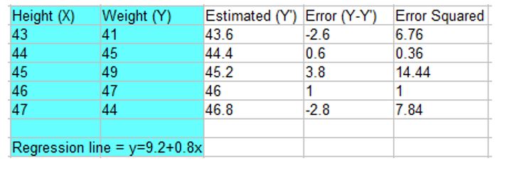
The data from the live page: five people with their height (X) and weight (Y). The page does not state the units, so treat them as plain numbers.
| Person | 1 | 2 | 3 | 4 | 5 |
|---|---|---|---|---|---|
| Height (X) | 43 | 44 | 45 | 46 | 47 |
| Weight (Y) | 41 | 45 | 49 | 47 | 44 |
Step 1: Find the Regression Line
The mean of X is 45 and the mean of Y is 45.2. The sum of (x minus x bar) times (y minus y bar) is 8.0, and the sum of (x minus x bar) squared is 10. So the slope is 8.0 divided by 10 = 0.8, and the intercept is 45.2 minus 0.8 times 45 = 9.2.
The regression line is Y’ = 9.2 + 0.8X. The live page gives this line without showing how it was found. I checked that it is the least squares line.
Step 2: Predict Y for Each X
Put each height into the line. For X = 44, Y’ = 9.2 + 0.8 times 44 = 44.4. Do the same for the others.
Step 3: Find the Error for Each Point
Error = Y minus Y’. For X = 44, the error is 45 minus 44.4 = 0.6.
Step 4: Square the Errors
For the same point, 0.6 squared = 0.36. The table gives all five.
| Height (X) | Weight (Y) | Predicted Y’ | Error (Y minus Y’) | Squared error |
|---|---|---|---|---|
| 43 | 41 | 43.6 | minus 2.6 | 6.76 |
| 44 | 45 | 44.4 | 0.6 | 0.36 |
| 45 | 49 | 45.2 | 3.8 | 14.44 |
| 46 | 47 | 46.0 | 1.0 | 1.00 |
| 47 | 44 | 46.8 | minus 2.8 | 7.84 |
| Total | 30.40 |
The live page lost its superscripts in this step. For example, it prints minus 2.62 = 6.76, where it means minus 2.6 squared = 6.76.
Step 5: Take the Mean
The mean squared error of this regression line is 6.08.
How to Read an MSE?
A single MSE is hard to judge on its own. Its unit is the square of your data’s unit, so it is not easy to picture. Use these steps.
Take the Square Root: RMSE
The root mean squared error is the square root of MSE. It is in the same unit as Y. Here RMSE = the square root of 6.08 = 2.47, so a typical prediction is off by about 2.5 weight units.
Compare with a Baseline
The simplest model ignores height and always predicts the average weight, 45.2. Its MSE is 36.8 divided by 5 = 7.36. Our line gets 6.08, so it beats the baseline, but only slightly. The R squared is 1 minus 30.4 divided by 36.8 = 0.17, which means that height explains only about 17 percent of the variation in weight in this small sample. A model is only as good as its gain over a simple baseline.
Compare Other Lines
The least squares line has the smallest possible MSE. Other lines do worse.
| Line | MSE |
|---|---|
| Y’ = 9.2 + 0.8X (least squares) | 6.08 |
| Y’ = X | 6.20 |
| Y’ = 30 + 0.3X | 9.47 |
MSE Divided by n, or n Minus 2?
In this tutorial, MSE divides by n. Some regression software reports a residual mean square that divides the sum of squared errors by n minus 2, since two values (a and b) are estimated. For these data that gives 30.4 divided by 3 = 10.13. When you read a report, check which one is meant.
MSE, RMSE and MAE
| Measure | Formula in words | Notes |
|---|---|---|
| MSE | The mean of squared errors | Punishes large errors. Unit is squared |
| RMSE | The square root of MSE | Same unit as Y. Easier to explain |
| MAE | The mean of absolute errors | Treats all errors alike. Less sensitive to outliers |
For our example, MSE is 6.08, RMSE is 2.47 and MAE is 2.16. To see the difference in sensitivity, take five errors that are all 1. MSE is 1 and MAE is 1. Change one error to 6, and MSE jumps to 8.0 while MAE only rises to 2.0. One large miss dominates MSE. That is useful when big errors are costly, and misleading when a few outliers are just noise.
Calculate MSE in Python
I ran the code below, and the output is real.
The results match the hand calculation. A caution: this is MSE on the same data that built the line, called training error. For real work, calculate MSE on test data that the model has not seen.
Common Mistakes to Avoid
| Mistake | Fix |
|---|---|
| Averaging the errors without squaring | Positive and negative errors cancel and hide the problem |
| Calling a result good without a baseline | Compare with predicting the mean |
| Reporting MSE in the unit of Y | MSE is in squared units. Use RMSE for the original unit |
| Judging the model only on training data | Use a test set |
| Mixing up the divide by n and the divide by n minus 2 versions | State which one you use |
| Letting one outlier mislead you | Check MAE and the residual plot |
Practice Questions
- A model makes errors of 2, minus 1, 3 and minus 2 on four points. Find the MSE.
- Find the RMSE for the MSE in question 1.
- A model has an MSE of 20 and a baseline that always predicts the mean has an MSE of 25. Is the model good?
- Why do we square the errors instead of just adding them?
Answers: 1) (4 + 1 + 9 + 4) divided by 4 = 4.5. 2) The square root of 4.5 = 2.12. 3) It beats the baseline, but only a little. An MSE of 20 against 25 means a modest gain, about 20 percent lower, so check R squared and other models before you rely on it. 4) Positive and negative errors would cancel, hiding the real size of the misses. These are my own answers, so please recheck them before publishing.
MSE turns a pile of prediction errors into one number, and it is also the quantity that decides which line gets chosen. Work through the five point example by hand, then do the same on your own data in Python. And always ask the follow up question: compared with what? A baseline gives an MSE its meaning.
