Z Score: Definition, Formula and Worked Examples

Sarah scores 70 out of 100. Is that good? It depends on the class. If the average was 60, she did well. If the average was 85, she did badly. A raw score means little until you compare it with the group. A z score does exactly that: it tells you how far a value sits from the average, counted in standard deviations.

It is one of the simplest and most used tools in data science. Analysts use it to compare values measured on different scales, to find outliers, to scale features before a model, and to turn a normal curve question into a table lookup.

This tutorial explains what a z score is, how to read positive and negative values, the formula, a fully worked example with the answer, how to find percentiles and work backwards, how to spot outliers, and how to calculate z scores in Python.

Z Score in Data Science: Definition

A z score, also called a standard score, shows how many standard deviations a data point lies from the mean of its group.

How to Read a Z Score?

• z = 0: the value equals the mean.
• z = 1: the value is one standard deviation above the mean.
• z = 2: two standard deviations above the mean.
• z = 3: three standard deviations above the mean. This is rare.
• A positive z: the value is above the mean.
• A negative z: the value is below the mean. For example, z = minus 1.5 is one and a half standard deviations below.

The size of z matters, not just its sign. A z of 2.4 and a z of minus 2.4 are equally far from the mean, on opposite sides.

The live page says that a z score comes under probability. It is calculated as part of descriptive statistics, where it is a way of standardizing data. It enters probability when you read the area under the normal curve for a z value.

Z Score Formula

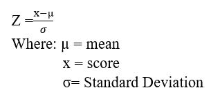
• x = the value you are checking.
• mean = the average of the group.
• standard deviation = the spread of the group.

In symbols, for a population: z = (x minus mu) divided by sigma. For a sample: z = (x minus x bar) divided by s.

Steps to Calculate a Z Score

1. Find the mean of the data.
2. Find the standard deviation.
3. Subtract the mean from the value.
4. Divide by the standard deviation.
5. Read the result: its sign gives the direction and its size gives the distance.

Z Score Example

Example 1: Sarah’s Score

The live page: Sarah scored 70 out of 100. The class mean was 60 and the standard deviation was 15. How many students scored higher or lower? The page does not answer. Here is the full solution.

• Z = (70 minus 60) divided by 15 = 10 divided by 15 = 0.667.
• Meaning: Sarah is about two thirds of a standard deviation above the class mean.
• Area to the left of 0.667 = 0.7475 (from a z table or software).

If the marks follow a normal distribution, about 74.75 percent of the class scored lower than Sarah, and about 25.25 percent scored higher. The normal assumption matters. Without it, the z score still tells you the distance from the mean, but the percentage may be different.

Example 2: Working Backwards

You can turn a z score back into a raw score: x = mean plus z times standard deviation.

• A z of 1.5 in Sarah’s class is a score of 60 + 1.5 times 15 = 82.5.
• The 90th percentile has a z of 1.282, so the score is 60 + 1.282 times 15 = 79.22. A student needs about 79 marks to beat 90 percent of the class.

Example 3: Comparing Two Exams

Exam A: the mean is 70, the standard deviation is 8, and a student scores 82. Exam B: the mean is 500, the standard deviation is 100, and a student scores 640.

The 82 is slightly stronger, at 1.5 standard deviations above its mean against 1.4. This is the main use of z scores: putting different scales on one ruler.

Example 4: A Small Class

Eight students scored 55, 60, 65, 70, 48, 72, 80 and 58. The mean is 63.5. The population standard deviation is 9.644, and the sample standard deviation is 10.309. Their z scores, using the population standard deviation, are:

Two things to notice. The z scores are negative for marks below the mean, and the 80 stands out most, at 1.71. And after standardizing, the z scores have a mean of 0 and a standard deviation of 1. Check the code below.

Population or sample? If your data are the whole group, divide by the population standard deviation. If they are a sample, the sample version, with n minus 1, is usually used. The z scores change a little. Python’s stats.zscore uses the population version unless you set ddof to 1.

Using Z Scores to Find Outliers

A common rule marks a value as an outlier if its z score is above 3 or below minus 3. For normal data, only about 0.27 percent of values lie that far out. In my test, I made 49 normal values with a mean of 60 and a standard deviation of 15, and added one extreme value, 140. Its z score was 4.18, and it was the only value with an absolute z score above 3.

A warning: an outlier raises the standard deviation, which makes its own z score smaller. In small data sets, extreme values can hide. Also, for skewed data, the rule of three can flag too many or too few points.

Z Score Table: Common Values

Calculate Z Scores in Python

I ran the code below, and the output is real.

import numpy as np
from scipy import stats

# Sarah: 70 out of 100, class mean 60, sd 15
z = (70 - 60) / 15
print("Sarah z:", round(z, 3))
print("Share who scored lower (normal data):", round(float(stats.norm.cdf(z)), 4))
print("Share who scored higher:", round(float(stats.norm.sf(z)), 4))

# Working backwards: score for z = 1.5 and for the 90th percentile
print("Score at z = 1.5:", 60 + 1.5 * 15)
print("Score at 90th percentile:", round(60 + float(stats.norm.ppf(0.90)) * 15, 2))

# A small class: marks of 8 students
marks = np.array([55, 60, 65, 70, 48, 72, 80, 58])
print("Mean:", marks.mean(), " Population sd:", round(float(marks.std()), 3), " Sample sd:", round(float(marks.std(ddof=1)), 3))
zs = stats.zscore(marks)
print("Z scores:", [round(float(v), 2) for v in zs])
print("Mean of z scores:", round(float(zs.mean()), 4), " sd of z scores:", round(float(zs.std()), 4))

# Spotting outliers: one extreme value among 50 normal values
rng = np.random.default_rng(4)
x = np.append(rng.normal(60, 15, 49), 140)
zz = stats.zscore(x)
print("Largest z:", round(float(zz.max()), 2), " Values with |z| above 3:", int((np.abs(zz) > 3).sum()))

# Comparing two exams
print("Exam A z:", round((82 - 70) / 8, 2), " Exam B z:", round((640 - 500) / 100, 2))

Sarah z: 0.667
Share who scored lower (normal data): 0.7475
Share who scored higher: 0.2525
Score at z = 1.5: 82.5
Score at 90th percentile: 79.22
Mean: 63.5  Population sd: 9.644  Sample sd: 10.309
Z scores: [-0.88, -0.36, 0.16, 0.67, -1.61, 0.88, 1.71, -0.57]
Mean of z scores: 0.0  sd of z scores: 1.0
Largest z: 4.18  Values with |z| above 3: 1
Exam A z: 1.5  Exam B z: 1.4

Common Mistakes to Avoid

Practice Questions

1. Mean 50, standard deviation 10. Find the z score of 68.
2. Mean 80, standard deviation 12. A z score is minus 1.5. What is the value?
3. A student has z = 2 in Exam A and z = 1.2 in Exam B. Which result is stronger?
4. A value has z = minus 3.4. Is it likely an outlier?

Answers: 1) (68 minus 50) divided by 10 = 1.8. 2) 80 + (minus 1.5) times 12 = 62. 3) Exam A, since 2 is higher than 1.2. 4) Yes, it is beyond minus 3, so check it. These are my own answers, so please recheck them before publishing.

A z score takes a raw number and gives it context: how far from the average, in which direction and in units that work everywhere. Learn the formula, remember that the sign gives the direction, and you can compare almost anything.