Sample Variance
Sample Variance: Formula, Examples and Why We Divide by n Minus 1
Two classes score an average of 70 marks in a test. In the first class, every student scored between 68 and 72. In the second, some scored 30 and others scored 100. The averages match, but the classes are nothing alike. The average alone hides this. You need a number that says how spread out the marks are, and variance is that number.
Variance is one of the first ideas in statistics for data science. It sits behind standard deviation, z scores, regression, and many machine learning methods. Most beginners can write the formula. Fewer know why the sample version divides by n minus 1 instead of n, and this is where wrong answers come from, including on the live version of this page.
In this tutorial you will learn what sample variance is, how to calculate it step by step on real numbers, how it differs from population variance, why the n minus 1 matters, and how to get the same answers in Python. You should know the mean first. If not, read our measures of central tendency tutorial.
What is Sample Variance?
Variance measures how far the values of a dataset spread out around their mean. A small variance means the values sit close to the mean. A large variance means they are scattered.
Sample variance is the variance of a sample, which is a smaller group taken from a larger population. You rarely measure a whole population, such as every customer or every machine part, so you measure a sample and use it to estimate the population. Sample variance is written as s squared.
| Aspect | Sample | Population |
|---|---|---|
| Symbol for variance | s squared | sigma squared |
| Symbol for the mean | x bar | mu |
| Count | n | N |
| Divide the sum of squares by | n minus 1 | N |
Sample Variance Formula
In symbols: s squared equals the sum of (xi minus x bar) squared, divided by (n minus 1). Here xi is each value, x bar is the sample mean, and n is the number of values.
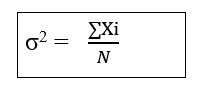
The standard deviation is the square root of the variance. It is in the same unit as your data, so it is easier to read. If the variance is in kilograms squared, the standard deviation is in kilograms.
How to Calculate Sample Variance? Step by Step
- Find the mean of the sample.
- Subtract the mean from each value. These are the deviations.
- Square each deviation. Squaring removes the minus signs, so positive and negative deviations do not cancel.
- Add the squared deviations.
- Divide the total by n minus 1.
The live page lists three steps, which are to square each item, add them, and divide by N. It skips the subtraction of the mean, and that is why its answer is wrong.
Worked Example 1: Ten Numbers
The data is 3, 5, 6, 4, 8, 10, 6, 7, 2, 1. There are 10 values, and they add up to 52, so the mean is 5.2.
| Value | Value minus mean | Squared deviation |
|---|---|---|
| 3 | minus 2.2 | 4.84 |
| 5 | minus 0.2 | 0.04 |
| 6 | 0.8 | 0.64 |
| 4 | minus 1.2 | 1.44 |
| 8 | 2.8 | 7.84 |
| 10 | 4.8 | 23.04 |
| 6 | 0.8 | 0.64 |
| 7 | 1.8 | 3.24 |
| 2 | minus 3.2 | 10.24 |
| 1 | minus 4.2 | 17.64 |
| Total | 0 | 69.6 |
The deviations always add up to zero around the mean. That is a useful check on your work. The squared deviations add up to 69.6.
- Sample variance = 69.6 divided by (10 minus 1) = 69.6 divided by 9 = 7.73
- Sample standard deviation = the square root of 7.73 = 2.78
- Population variance, if these 10 numbers were the whole population: 69.6 divided by 10 = 6.96
The live page gets 34 for this data. It squares the raw values (9, 25, 36 and so on), adds them to 340, and divides by 10. That number is the average of the squares, which is not the variance. There is a shortcut that does use 340, and it gives the right answer: the sum of squares of the values minus n times the mean squared, which is 340 minus 10 times 5.2 squared = 340 minus 270.4 = 69.6. It is the same result as above, but it needs that subtraction.
Worked Example 2: Weights in Kilograms
Seven workers at a plant are weighed for a safety harness fitting. Their weights in kilograms are 58, 62, 65, 70, 72, 75 and 80. The mean is 68.86 kg. Following the same steps, the sample variance is 58.81 and the standard deviation is 7.67 kg. A rough reading is that a typical worker sits about 7.7 kg from the mean of 68.9 kg. This is my own example and I ran the numbers in Python, so it replaces the weights example on the live page.
Why Divide by n Minus 1?
This is the question to understand. When you only have a sample, you do not know the true population mean. You use the sample mean, which by its nature sits closer to your sample values than the true mean does. So the deviations around it come out a little too small, and dividing by n understates the true variance. Dividing by n minus 1 corrects for that. This is called Bessel’s correction. One way to say it is that one degree of freedom is used up to estimate the mean.
You can see this with a simulation. I created a population of one million values with a true variance of about 100. Then I took 20,000 random samples of size 5 from it, and calculated the variance for each in two ways.
| Method | Average result |
|---|---|
| True population variance | 100.1 |
| Divide by n (average over 20,000 samples) | 80.5 |
| Divide by n minus 1 (average over 20,000 samples) | 100.7 |
Dividing by n lands near 80, which is the true value times (n minus 1) divided by n, or 4 divided by 5. Dividing by n minus 1 lands near the true value. The small difference from 100.1 is random variation in the simulation. The correction matters most when the sample is small. With 1000 values, n and n minus 1 are almost the same.
One caveat. The square root of an unbiased variance is still slightly biased downward, so the sample standard deviation is not perfectly unbiased. For most work this is ignored. Also, with only one value (n = 1), a sample variance cannot be calculated, because you would divide by zero.
Calculate Sample Variance in Python
Here is the same example in code. I ran it, and the output is real. Watch the defaults. The statistics module and pandas divide by n minus 1, but NumPy divides by n unless you set ddof to 1. This difference causes many silent errors.
| Library | Sample variance (n minus 1) | Population variance (n) |
|---|---|---|
| statistics | variance() | pvariance() |
| NumPy | np.var(x, ddof=1) | np.var(x), the default |
| pandas | Series.var(), the default | Series.var(ddof=0) |
Where Sample Variance is Used in Data Science
- Checking data quality. A column with zero variance holds one value, so it adds nothing to a model.
- Comparing groups. Two machines can produce parts with the same average length, but the one with the lower variance is more consistent.
- Feature scaling. Standardisation divides by the standard deviation, which comes from variance.
- Hypothesis tests and confidence intervals. The T test and ANOVA both use sample variance.
- Risk. In finance, the variance of returns is a basic measure of risk.
Common Mistakes to Avoid
| Mistake | Fix |
|---|---|
| Squaring the raw values instead of the deviations | Subtract the mean first |
| Dividing by n for a sample | Divide by n minus 1 |
| Mixing the symbols s squared and sigma squared | Use s squared for samples and sigma squared for populations |
| Using np.var and assuming it is the sample version | Set ddof=1 |
| Quoting variance as if it had the data’s unit | It is in squared units. Use the standard deviation to speak in the original unit |
| Calculating variance for one value | You need at least two values |
Practice Questions
- Find the sample variance of 4, 8, 6, 5, 2.
- The sum of squared deviations of a sample of 8 values is 56. Find the sample variance and the sample standard deviation.
- Why can you not calculate a sample variance from one value?
Answers: 1) Mean 5, deviations minus 1, 3, 1, 0, minus 3, squares 1, 9, 1, 0, 9, total 20, divided by 4 gives 5. 2) 56 divided by 7 = 8, and the square root is about 2.83. 3) The mean equals the value, the sum of squares is zero, and n minus 1 is zero, so you divide by zero. I calculated these by hand, so please recheck them.
Variance is easy to calculate and easy to get wrong. Remember the three habits: subtract the mean first, divide by n minus 1 for a sample, and check which default your library uses. Try the practice questions, then run the same numbers in Python to confirm.
