Two Tailed Test
Two Tailed Test: Definition, Formula and Worked Examples
A factory says that its bolts are 70 millimetres long. You measure a sample and find an average of 71.9. Is the factory off target? It could be producing bolts that are too long, but it could just as well produce bolts that are too short. If you only watch for one direction, you can miss the problem in the other. A two tailed test watches both.
It is the default hypothesis test in research and data science. A and B tests, quality checks and medical trials are usually two tailed, because you want to know if anything changed, not only if something went up. The name sounds technical, but the idea is simple: the rejection area is split between the two ends, or tails, of a curve.
This tutorial explains what a two tailed test is, why and when to use it, the formula, the cut off values, two worked examples with every step shown, how it differs from a one tailed test, and how to run it in Python. You should know what a null hypothesis and a p value are, and have some idea of the normal curve.
Two Tailed Test Definition
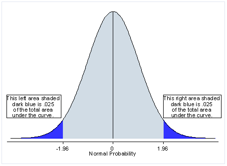
A two tailed test is a hypothesis test in which the rejection region lies in both tails of the sampling distribution. You reject the null hypothesis if your test statistic is either very low or very high. The test is used when the alternative hypothesis says that a value is different, without saying in which direction.
At a 5 percent significance level, the 5 percent is split in two: 2.5 percent in the left tail and 2.5 percent in the right tail. On the standard normal curve, the cut off values are minus 1.96 and plus 1.96. If your Z value falls beyond either of them, you reject the null hypothesis.
| Significance level (alpha) | Area in each tail | Critical Z values |
|---|---|---|
| 0.10 | 0.05 | Minus 1.645 and plus 1.645 |
| 0.05 | 0.025 | Minus 1.960 and plus 1.960 |
| 0.01 | 0.005 | Minus 2.576 and plus 2.576 |
The live page calls these Z cut offs a standard deviation value. They are Z values, which count the number of standard errors from the mean.
Why do We Use a Two Tailed Test?
You use it for a non directional hypothesis, one that says there is a difference, not that the value is higher or lower.
- Null hypothesis, H0: the mean is 70.
- Alternative hypothesis, H1: the mean is not 70, so it may be less than or more than 70.
The advantage is that it catches changes in both directions. It protects you when you do not know which way the effect will go, or when a change either way is a problem, as with the bolt length. The cost is that it is harder to reach significance, because the 5 percent of risk is spread over two tails.
In symbols: H0: mu = mu0, and H1: mu is not equal to mu0. The live page writes the alternative as H1<>, which may not display on all screens.
The Two Tailed Test Formula
For a test of a mean with a known population standard deviation (a Z test):
The bottom part, the standard deviation divided by the square root of n, is the standard error. The live page prints it with the square root part missing.
The p value for a two tailed test counts both tails:
How to Use a Two Tailed Test? Step by Step
- State the hypotheses. H0: the mean equals the hypothesised value. H1: it does not.
- Choose the significance level, alpha, such as 0.05. Do this before looking at the data.
- Find the critical values. For 0.05, they are minus 1.96 and plus 1.96.
- Calculate the test statistic, Z or t.
- Decide. Reject H0 if the statistic is beyond a critical value, or if the p value is below alpha.
- State the conclusion in plain words.
Example 1: Brokerage Fees
The live page: the average brokerage fee in the population is 22 dollars, with a standard deviation of 9. A sample of 600 accounts has a mean of 15 dollars and a standard deviation of 9. Is the sample different from the population?
- Hypotheses. H0: the mean fee is 22. H1: the mean fee is not 22. The live page sets H0 to 15, which is the sample mean. A null hypothesis is about the population, so it must be 22.
- Alpha = 0.05. The critical values are minus 1.96 and plus 1.96.
- Standard error = 9 divided by the square root of 600 = 0.3674.
- Z = (15 minus 22) divided by 0.3674 = minus 19.05.
- Decision. Minus 19.05 is far below minus 1.96. The p value is about 6 times 10 to the power minus 81, which is below 0.05.
Conclusion: we reject the null hypothesis. The sample fees are different from the population average, and with a mean of 15 against 22, they are lower. The live page concludes that there is not enough evidence of a difference, which does not follow from its own numbers. If the claim was only that the fees are lower, a one tailed test would also fit. Here the answer is the same.
Two Tailed Test Example 2
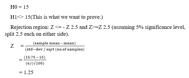
The live page: the hypothesised mean is 18, the sample mean is 18.75, and the standard deviation is 6. It never gives n, and it mixes the null values 15 and 18. I use H0: the mean is 18, and a sample size of 100. The value 100 is my assumption, and it is the only n for which the page’s Z of 1.25 works.
- Hypotheses. H0: the mean is 18. H1: the mean is not 18.
- Standard error = 6 divided by the square root of 100 = 0.6.
- Z = (18.75 minus 18) divided by 0.6 = 1.25.
- Critical values at 0.05: minus 1.96 and plus 1.96. The value 1.25 lies between them, so it is not in the rejection region.
- p value = 2 times P(Z greater than 1.25) = 2 times 0.1056 = 0.2113. This is above 0.05.
Conclusion: we do not reject the null hypothesis. There is not enough evidence that the mean differs from 18. A 95 percent interval for the true mean runs from 17.57 to 19.93, which contains 18. This agrees with the test, because a two tailed test at 0.05 and a 95 percent interval always agree.
What Happens with More Data?
The same gap of 0.75 looks different with a bigger sample. With n = 400, the standard error is 0.3, Z = 2.50 and the two tailed p value is 0.0124, which is significant. Not significant here means that we do not have enough data. It does not mean that the difference is zero.
Two Tailed vs One Tailed Test
| Point | Two tailed | One tailed |
|---|---|---|
| Alternative hypothesis | Different from the value, in either direction | Greater than, or less than, the value, in one direction |
| Rejection region | Both tails, 2.5 percent each at alpha 0.05 | One tail, 5 percent at alpha 0.05 |
| Critical Z at 0.05 | Minus 1.96 and plus 1.96 | 1.645 in the direction you chose |
| p value | Both tails counted, twice the one tail area | One tail area |
| Use when | Any change matters, or you have no strong reason to expect a direction | Only one direction matters, decided before the data |
For Example 2, the one tail area is 0.1056, so a one tailed test would give a p value of 0.1056, which is still not significant.
Why the Choice Must Be Made Before You See the Data?
Here is a case in which the choice matters. Twelve bolts measure 68, 72, 75, 66, 74, 71, 73, 69, 77, 70, 76 and 72 millimetres. The mean is 71.92 and the target is 70. A one sample T test gives t = 2.00.
| Test | p value |
|---|---|
| Two tailed, H1: the mean is not 70 | 0.0705, not significant |
| One tailed, H1: the mean is greater than 70 | 0.0352, significant |
The one tailed test looks stronger, because it puts all 5 percent in one tail. But if you pick the direction after seeing that the mean is above 70, you are cheating, and you double your real false positive rate. Use a one tailed test only if the direction was fixed before the data, for a good reason. When in doubt, use two tailed.
Run a Two Tailed Test in Python
I ran the code below, and the output is real.
In SciPy, the alternative argument chooses the type of test. Two sided is the default for the T test functions.
Common Mistakes to Avoid
| Mistake | Fix |
|---|---|
| Setting the null hypothesis to the sample mean | The null hypothesis is a claim about the population |
| Forgetting to double the one tail area for the p value | A two tailed p value counts both tails |
| Choosing one tailed after seeing the data | Fix the direction before the test |
| Using the one tailed cut off 1.645 in a two tailed test | Use 1.96 at alpha 0.05 |
| Concluding that no difference exists when p is high | It means not enough evidence |
| Leaving out the sample size | Report n, because it sets the standard error |
| Mixing the null values in different parts of a problem | Use one H0 throughout |
Practice Questions
- At alpha 0.05, what are the critical Z values for a two tailed test?
- A Z value of 2.30 is found. Is it significant in a two tailed test at 0.05?
- The area to the right of Z = 1.80 is 0.0359. What is the two tailed p value?
- When would you use a one tailed test?
Answers: 1) Minus 1.96 and plus 1.96. 2) Yes, because 2.30 is greater than 1.96. 3) 2 times 0.0359 = 0.0718, which is not significant at 0.05. 4) When only one direction matters and it was decided before seeing the data. These are my own answers, so please recheck them before publishing.
A two tailed test asks a simple question: is the value different from what I expected, in either direction? Decide the hypotheses and alpha before you see the data, use the cut off values of minus and plus 1.96 at 0.05, and double the one tail area for the p value. That habit keeps your results honest.
