Law of Large Numbers
Law of Large Numbers: Definition, Formula and Examples
Roll a die three times and you may get 6, 6 and 3. The average is 5, far from the 3.5 you would expect. Roll it a hundred thousand times and the average sits within 0.01 of 3.5. This is the law of large numbers at work: the more data you collect, the closer the average gets to the truth.
It sounds obvious, but it is the reason that surveys, insurance, casinos and A and B tests work at all. It is also one of the most misunderstood ideas. People use it to claim that tails is due after five heads. It says no such thing, and this tutorial shows why with real simulations.
You will learn what the law says, the formula, two worked examples with all the numbers, how fast the error shrinks, the gambler’s fallacy, how the law differs from the central limit theorem, and how to simulate it in Python.
Law of Large Numbers Definition
The law of large numbers says that if you repeat an independent experiment many times and average the results, the average will get close to the expected value. In other words, as the sample size grows, the sample mean gets closer to the population mean.
In symbols, let X1 to Xn be independent values with the same expected value mu, and let x bar be their average. Then:
The expected value is the long run average of a random outcome, each value weighted by its probability. For a fair die it is (1 + 2 + 3 + 4 + 5 + 6) divided by 6 = 3.5, a number that no single roll can show.
What the law does not say. It does not promise that a small sample reflects the population. It does not say that early bad luck is cancelled out by later luck. It says that the average of the whole sample gets close to the truth because the early results get diluted by many more.
Weak and Strong Law
There are two versions. The weak law says that the chance of a large gap goes to zero. The strong law says that the sample mean will, with probability 1, end up at the expected value. For everyday use, the idea is the same.
Why do We Need the Law of Large Numbers in Statistics?
- Surveys. You cannot ask everyone, so you ask a sample. The law says that a bigger sample gives an average nearer the truth.
- Estimation. It is the reason why the sample mean is a sensible estimate of the population mean.
- Business with risk. Insurers and casinos earn steady results because they handle huge numbers of independent events.
- Testing. A and B tests collect data until the averages settle.
You may not be able to survey everyone, but each extra data point makes your result more likely to be close to the true mean.
Example of the Law of Large Numbers
Example 1: Drawing Numbers from 1 to 100
The data set is the whole numbers from 1 to 100. The true average is 50.5. The live page draws two values, 95 and 40, and gets (95 + 40) divided by 2 = 67.5, and says that more draws should move the average toward the true value. It never states 50.5, so here it is. I ran a simulation of random draws.
| Number of draws | Average | Gap from 50.5 |
|---|---|---|
| 2 | 82.00 | 31.50 |
| 20 | 47.35 | 3.15 |
| 200 | 47.27 | 3.23 |
| 20,000 | 50.37 | 0.13 |
Notice that 200 draws were not closer than 20 draws. The law says that large samples are close with high probability. It does not say that every step gets closer. With 20,000 draws, the average is very near 50.5.
Example 2: Rolling a Die
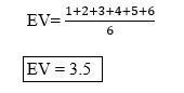
A fair die has six equally likely faces, and the expected value is 3.5. The live page shows three rolls: 6, 6 and 3. The average is (6 + 6 + 3) divided by 3 = 5, far from 3.5. Here is what happens as I keep rolling in a simulation.
| Number of rolls | Average | Gap from 3.5 |
|---|---|---|
| 3 | 3.333 | 0.167 |
| 10 | 3.200 | 0.300 |
| 100 | 3.570 | 0.070 |
| 1,000 | 3.471 | 0.029 |
| 10,000 | 3.517 | 0.017 |
| 100,000 | 3.508 | 0.008 |
The average wiggles at first, then settles. The simulation gave a different first three rolls than 6, 6, 3, but the pattern is the same.
How Fast does the Error Shrink?
The typical error of an average falls with the square root of n. I repeated the die experiment 2,000 times for each size and measured the average gap from 3.5.
| Rolls per average | Typical error | Compared with n = 10 |
|---|---|---|
| 10 | 0.444 | Base |
| 100 | 0.140 | About a third |
| 1,000 | 0.043 | About a tenth |
A hundred times the data gives a tenth of the error. The standard error formula, sigma divided by the square root of n, explains it.
The Gambler’s Fallacy: What the Law does Not Say?
After five heads in a row, many people feel that tails is due. The law of large numbers does not say that. Coin flips have no memory. I tested it: in 2,000,000 simulated flips, there were 63,478 streaks of five heads, and the next flip was heads 50.46 percent of the time.
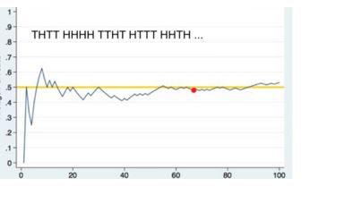
Here is how the law really works. It is the share of heads that settles near one half, not the difference between heads and tails. In my 100,000 flips, the heads minus tails gap was minus 4 after 100 flips, and 164 after 10,000, but the share of heads went to 0.4992 after 100,000 flips. The gap in counts can grow while the share gets close to 0.5, because the early results are diluted, not corrected.
| Flips | Share of heads | Heads minus tails | Closer to 0.5? |
|---|---|---|---|
| 10 | 0.5000 | 0 | Yes |
| 100 | 0.4800 | Minus 4 | Not yet |
| 10,000 | 0.5082 | 164 | Yes |
| 100,000 | 0.4992 | Minus 154 | Yes |
A Biased Sample is Not Fixed by Size
The law needs independent samples from the same population. If your survey asks only the people who walk into one shop, a million answers will converge to the wrong value. More data cannot repair a biased sample.
Law of Large Numbers vs Central Limit Theorem
| Point | Law of large numbers | Central limit theorem |
|---|---|---|
| Question | Where does the average end up? | What shape does the spread of the average have? |
| Answer | At the expected value | A normal curve with standard deviation sigma divided by the square root of n |
| Gives | Confidence that a big sample is close | A way to compute how close, and the probability |
The law tells you that the average will settle. The central limit theorem tells you how it wobbles on the way.
A Different Meaning in Business
The live page notes that in business, the law of large numbers has another use: a very large firm cannot keep a high growth rate forever. This is a different idea from the statistical law, and it is better to treat them as two separate topics.
Simulate the Law of Large Numbers in Python
I ran the code below, and the output is real.
Common Mistakes to Avoid
| Mistake | Fix |
|---|---|
| Thinking tails is due after a streak of heads | Each flip is independent. The next one is still 50 percent |
| Expecting a small sample to match the population | The law needs a large sample |
| Expecting the difference in counts to shrink | Only the share, or the average, gets close |
| Thinking more data fixes a biased sample | Size cannot cure bias |
| Expecting every extra draw to get closer | The path wiggles. The trend is what counts |
| Mixing the law of large numbers with the central limit theorem | One is about the centre, the other about the shape |
| Mixing the statistical law with the business growth idea | They are different ideas |
Practice Questions
- What is the expected value of one roll of a fair die?
- The numbers 1 to 100 are the population. What is the true average?
- A coin has landed heads six times in a row. What is the probability that the next flip is heads?
- If the typical error with 100 values is 0.14, about what is it with 10,000 values?
Answers: 1) 3.5. 2) 50.5. 3) 0.5, since each flip is independent. 4) About 0.014, a tenth, since the error shrinks with the square root of n. These are my own answers, so please recheck them before publishing.
The law of large numbers is a promise about averages, not about the next outcome. Collect enough independent data and the average settles near the truth, slowly, with the square root of n. Do not expect a streak to correct itself, and do not expect size to cure a biased sample.
