Random Variable
Random Variable: Definition, Types and Examples for Beginners
You toss a coin five times. Before you start, you cannot say how many heads you will get. It could be none, it could be all five. But you can say something exact about the chances: the chance of exactly three heads is 10 out of 32. A random variable is the tool that lets you write this kind of statement cleanly.
It is one of the first ideas in probability, and almost everything after it depends on it. Probability distributions, expected value, the normal curve, hypothesis tests, and the models behind machine learning are all built on random variables. If this idea is shaky, the later topics feel like memorising rules.
In this tutorial, you will learn what a random variable is in plain words, the two types, discrete and continuous, with worked examples, how to find probabilities, the expected value and the variance, and how to check your work in Python. The only background needed is the basic idea of probability.
What is a Random Variable?
A random variable is a rule that gives a number to each possible outcome of a random experiment. It is usually written as a capital letter such as X. The experiment is random, so you do not know in advance which number you will get. You do know the set of possible numbers and how likely each one is.
Take one toss of a coin. The outcomes are Head and Tail. These are not numbers. Define X as 1 for a head and 0 for a tail, and now X is a random variable. Or toss the coin five times and define X as the number of heads. Now X can be 0, 1, 2, 3, 4 or 5.
How It Differs from a Variable in Algebra
In algebra, 12 plus x = 13 gives one fixed answer, x = 1. A random variable does not have one answer. It has a set of possible values, each with a probability. You cannot solve for it. You describe it.
The Notation
| Notation | Meaning |
|---|---|
| X | The random variable, a capital letter |
| x | One possible value of X, a small letter |
| P(X = 3) | The probability that X takes the value 3 |
| P(X < 4) | The probability that X is less than 4 |
| E(X) | The expected value, or mean, of X |
This short form is the main benefit. Instead of writing the probability of getting fewer than four heads in five tosses, you write P(X < 4).
Different Types of Random Variables
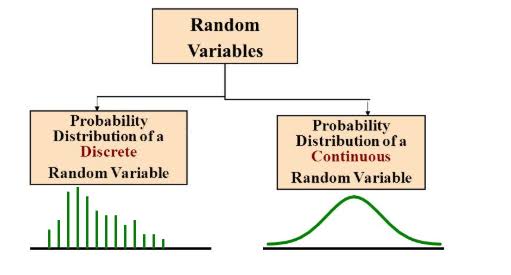
There are two types, and the difference decides which tools you use.
| Feature | Discrete | Continuous |
|---|---|---|
| Values | Countable, separate values | Any value in a range, including decimals |
| Examples | Number of heads, defects in a batch, calls per hour | Height, weight, time, temperature |
| Probability of one exact value | Can be more than zero | Always zero |
| Described by | Probability mass function | Probability density function |
| Probability of a range | Add the probabilities | Find the area under the curve |
Discrete Random Variable
A discrete random variable takes values you can list and count, such as 0, 1, 2 and so on. There are gaps between the values. You cannot have 2.5 heads.
Discrete Random Variable Example: Five Coin Tosses
Toss a fair coin five times. Let X be the number of heads. There are 2 times 2 times 2 times 2 times 2 = 32 equally likely outcomes. The number of ways to get k heads is the number of ways to choose k tosses from five. This gives the table below, called a probability distribution.
| x (heads) | Ways out of 32 | P(X = x) | As a decimal |
|---|---|---|---|
| 0 | 1 | 1 out of 32 | 0.03125 |
| 1 | 5 | 5 out of 32 | 0.15625 |
| 2 | 10 | 10 out of 32 | 0.3125 |
| 3 | 10 | 10 out of 32 | 0.3125 |
| 4 | 5 | 5 out of 32 | 0.15625 |
| 5 | 1 | 1 out of 32 | 0.03125 |
| Total | 32 | 32 out of 32 | 1 |
The probabilities add up to 1, as they must. Now the three questions that the live page leaves open:
- P(X = 3) = 10 out of 32 = 0.3125
- P(X < 4) means 0, 1, 2 or 3 heads. That is (1 plus 5 plus 10 plus 10) out of 32 = 26 out of 32 = 0.8125
- P(X > 1) means 2, 3, 4 or 5 heads. That is (10 plus 10 plus 5 plus 1) out of 32 = 26 out of 32 = 0.8125
A shortcut: P(X > 1) is 1 minus P(X = 0) minus P(X = 1), which is 1 minus 6 out of 32 = 26 out of 32. Using the opposite event often saves work.
Expected Value and Variance
The expected value is the long run average. You multiply each value by its probability and add the results: E(X) = the sum of x times P(X = x). For the five tosses it is 2.5. Of course you can never get 2.5 heads in one go. It is the average you would see over many sets of five tosses. The variance, which measures spread, is 1.25, and the standard deviation is about 1.12.
Another Discrete Example: Two Dice
Roll two fair dice and let X be the sum. X can be 2 to 12, but the values are not equally likely. There is one way to get a 2, six ways to get a 7, and one way to get a 12, out of 36 equally likely rolls.
| Sum | 2 | 3 | 4 | 5 | 6 | 7 |
|---|---|---|---|---|---|---|
| Ways out of 36 | 1 | 2 | 3 | 4 | 5 | 6 |
| Sum | 8 | 9 | 10 | 11 | 12 |
|---|---|---|---|---|---|
| Ways out of 36 | 5 | 4 | 3 | 2 | 1 |
The expected sum is 7. P(X is 10 or more) is (3 plus 2 plus 1) out of 36 = 6 out of 36, which is one in six.
Continuous Random Variable
A continuous random variable can take any value in a range, with no gaps. Height, time and temperature are of this kind. Between 170 cm and 171 cm there are endless possible values.
Continuous Random Variable Example: Heights
The live page uses basketball players between 4 and 7 feet. That range is arbitrary, so let us use a cleaner case. Suppose the heights of adult men in a group follow a normal curve with a mean of 170 cm and a standard deviation of 10 cm. These two numbers are my assumption for teaching, not real data.
Here is the surprise. The probability that someone is exactly 170 cm tall, to infinite precision, is zero. Nobody is exactly 170.00000 cm. So for a continuous variable we ask about ranges.
| Question | Probability |
|---|---|
| P(160 < X < 180) | 0.6827 |
| P(X > 190) | 0.0228 |
| P(X = 170 exactly) | 0 |
The first one is the 68 percent of the 68 95 99.7 rule, because 160 and 180 are one standard deviation from the mean. The second is the share of people more than two standard deviations above the mean. These were calculated with SciPy.
Density is Not Probability
A continuous variable has a probability density function. At 170 cm, the density is 0.0399. This is not the probability of 170 cm. The probability of a range is the area under the curve across that range. Beginners mix these up all the time.
Why Random Variables Matter in Data Science?
- Modelling uncertainty. Customer arrivals, defects and delivery times are random variables with a distribution.
- Describing data. The mean and the standard deviation of a column are estimates of the expected value and the spread of a random variable.
- Testing ideas. Hypothesis tests ask how likely a result is under a distribution.
- Machine learning. Many models, such as naive Bayes and linear regression with noise, assume particular distributions.
Check It in Python
You can verify the coin table with a few lines. I ran this code, and the output is real.
Python shows 5 out of 16 and 13 out of 16, which are the same as 10 out of 32 and 26 out of 32 in simplest form.
Common Mistakes to Avoid
| Mistake | Fix |
|---|---|
| Calling an outcome such as Head a random variable | Give it a number, such as 1 for head, or count heads |
| Treating the probabilities as not needing to add to 1 | They must total 1 for a complete distribution |
| Asking for the probability of one exact value of a continuous variable | Ask about a range |
| Mixing up density with probability | Probability is the area under the curve |
| Using plain counts when outcomes are not equally likely | Use the probability of each value, as with two dice |
| Expecting E(X) to be a value that X can take | It is an average and need not be a possible value |
Practice Questions
- A fair coin is tossed twice. Let X be the number of heads. Write the probability distribution.
- Roll one fair die. Let X be the number shown. Find E(X).
- Is the number of customers who visit a shop in an hour discrete or continuous? And the time a customer waits?
Answers: 1) P(X = 0) = 1 out of 4, P(X = 1) = 2 out of 4, P(X = 2) = 1 out of 4. 2) E(X) = (1 plus 2 plus 3 plus 4 plus 5 plus 6) divided by 6 = 3.5. 3) The number of customers is discrete, and the waiting time is continuous. These are my own answers, so please recheck them before publishing.
A random variable turns messy random outcomes into numbers you can work with. Start with the coin table, check the answers in Python, and then try the dice. Once discrete and continuous feel clear, the normal distribution and hypothesis tests will make far more sense.
