Probability Distribution Tutorial
Probability Distribution Tutorial for Beginners
A shop owner wants to stock enough items for tomorrow. She cannot know exactly how many customers will come, but she knows that on most days she gets two or three complaints, and on a few days none. That pattern, every possible result with how likely it is, is a probability distribution. It turns I do not know into I know the odds.
Probability distributions sit at the centre of data science. Every statistical test, every confidence interval and many machine learning models assume that data comes from some distribution. If you understand this idea, later topics such as the normal curve, hypothesis tests and regression become much easier to follow.
In this tutorial, you will learn what probability is, what a probability distribution is, the one rule that every distribution must follow, a worked bouquet example, how to find the expected value, the difference between discrete and continuous distributions, a map of the common ones, and how to check it in Python.
How are Probability and Statistics Used in Data Science?
Data science works with data that has noise and uncertainty. Statistics is the set of tools for describing and learning from such data, and probability is the language that statistics is written in. When a model says a customer has a 70 percent chance of leaving, that is probability. When you decide whether a new website design really beat the old one, you use the distribution of results you would expect by chance.
- Predicting. Models output probabilities, such as the chance that an email is spam.
- Testing. A hypothesis test asks how likely a result is if nothing special is going on.
- Simulating. You draw random numbers from a distribution to test ideas before real work.
- Describing. The mean and standard deviation of your data describe its distribution.
What is Probability?
Probability measures how likely an event is in a random experiment. A random experiment is one whose result you cannot predict for sure, such as tossing a coin or picking a flower. A probability runs from 0 to 1. A value of 0 means the event cannot happen, and 1 means it will certainly happen. It is calculated, not guessed.
Example: toss a fair coin. There are 2 possible outcomes and 1 of them is a head, so P(head) = 1 divided by 2 = 0.5.
What is a Probability Distribution?
A probability distribution describes all the possible values of a random variable, and how likely each one is. It can be shown as a table, a formula or a graph.
It must follow two rules.
- Every probability is between 0 and 1, including 0 and 1.
- All the probabilities add up to exactly 1, because one of the outcomes must happen.
If you are not sure what a random variable is, read our random variable tutorial first. In short, it is a rule that turns each outcome of an experiment into a number.
Formula of Probability Distribution
For a discrete random variable X, the distribution is given by P(X = x) for each possible value x, with two conditions: each P(X = x) is at least 0, and the sum of P(X = x) over all x equals 1.
When all outcomes are equally likely, P(X = x) = 1 divided by the number of outcomes, or more generally the number of ways x can occur divided by the total number of outcomes.

Probability Distribution Example: The Bouquet
A bouquet holds 10 red roses, 8 orchids, 10 blue roses and 12 lilies. That makes 40 flowers. You pick one flower without looking. What is the probability of each type?
| Flower | Count | Probability | As a percent |
|---|---|---|---|
| Red rose | 10 | 10 out of 40 = 0.25 | 25 percent |
| Orchid | 8 | 8 out of 40 = 0.20 | 20 percent |
| Blue rose | 10 | 10 out of 40 = 0.25 | 25 percent |
| Lily | 12 | 12 out of 40 = 0.30 | 30 percent |
| Total | 40 | 1.00 | 100 percent |
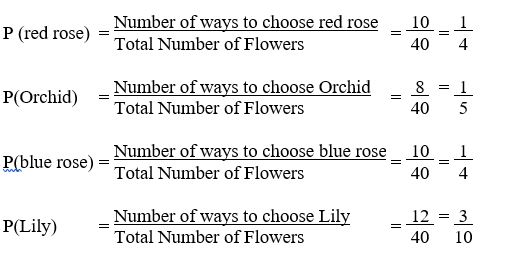
The table is a probability distribution, because every probability is between 0 and 1 and they add up to 1. Reading it, the lily is the most likely pick at 30 percent, and the orchid is the least likely at 20 percent. The live page says that the red and blue roses are the least likely, which is not right, since each has a higher chance than the orchid.
Now you can answer other questions by adding probabilities. The chance of picking any rose, red or blue, is 0.25 plus 0.25 = 0.50. The chance of not picking a lily is 1 minus 0.30 = 0.70.
A Number Based Example: Complaints per Day
The bouquet has categories. Most data science uses numbers, so here is a numeric one. This is my own example, with made up probabilities, for the number of complaints a shop gets in a day.
| Complaints (x) | P(X = x) |
|---|---|
| 0 | 0.10 |
| 1 | 0.30 |
| 2 | 0.35 |
| 3 | 0.20 |
| 4 | 0.05 |
| Total | 1.00 |
The probabilities add up to 1, so it is a valid distribution. Two complaints is the most likely day, at 0.35.
Expected Value and Spread
The expected value is the long run average. Multiply each value by its probability and add them. Here it is 0 times 0.10 plus 1 times 0.30 plus 2 times 0.35 plus 3 times 0.20 plus 4 times 0.05 = 1.8 complaints a day. The variance is 1.06, and the standard deviation is 1.03. In plain terms, a typical day has about 1.8 complaints, give or take one.
Cumulative Probability
A cumulative probability adds up the distribution to a point. The chance of at most 1 complaint is 0.10 plus 0.30 = 0.40. The running totals are 0.10, 0.40, 0.75, 0.95 and 1.00. The chance of 3 or more complaints is 0.20 plus 0.05 = 0.25.
Discrete and Continuous Distributions
| Aspect | Discrete | Continuous |
|---|---|---|
| Values | Countable, such as 0, 1, 2 | Any value in a range, such as height |
| Examples | Complaints per day, heads in 5 tosses, the bouquet | Height, time, temperature |
| Probability of one exact value | Can be above zero | Zero |
| Shown as | A table or bars, called a probability mass function | A smooth curve, called a probability density function |
| Probability of a range | Add the probabilities | Area under the curve |
Common Probability Distributions
You do not need to build every distribution from scratch. A few standard ones cover most real situations.
| Distribution | Type | Typical use |
|---|---|---|
| Uniform | Discrete or continuous | Every outcome equally likely, such as a die roll or a random number |
| Binomial | Discrete | Number of successes in a fixed number of yes or no trials, such as connected calls |
| Poisson | Discrete | Number of events in a fixed period, such as complaints per hour |
| Normal | Continuous | Values clustered around an average, such as heights and measurement errors |
Our uniform and binomial tutorials explain two of these in detail.
Check It in Python
I ran the code below, and the output is real.
A simulation of 100,000 random picks from the bouquet gave 0.249, 0.200, 0.251 and 0.300, very close to the exact values.
Common Mistakes to Avoid
| Mistake | Fix |
|---|---|
| Probabilities that add up to more or less than 1 | Check the total. It must be exactly 1 |
| Calling probability guesswork | It is a calculated measure of likelihood |
| Confusing probability with a distribution | A distribution lists the probability of every outcome |
| Reading the largest count as the biggest probability without dividing by the total | Divide by the total first |
| Asking for the probability of an exact value of a continuous variable | Ask for a range |
| Using the equally likely formula when outcomes are not equally likely | Use the real probability of each outcome |
Practice Questions
- Is this a valid probability distribution? P(1) = 0.2, P(2) = 0.5, P(3) = 0.4.
- Using the complaints table, find the probability of at most 1 complaint.
- In the bouquet, what is the probability of not picking an orchid?
- Find the expected value of one roll of a fair die.
Answers: 1) No, the probabilities add up to 1.1, not 1. 2) 0.10 plus 0.30 = 0.40. 3) 1 minus 0.20 = 0.80. 4) (1 plus 2 plus 3 plus 4 plus 5 plus 6) divided by 6 = 3.5. These are my own calculations, so please recheck them before publishing.
A probability distribution is simply the full picture of what could happen and how likely each case is. Build a few by hand, as in the bouquet and complaints examples, check that they add up to 1, and then move on to the named distributions.
