Sampling Distribution of the Sample Mean: Definition, Formula and Examples

Ask 20 athletes their height and you get an average. Ask another 20 and you get a slightly different average. Ask a third group and the number moves again. Which one is right? None of them exactly, and all of them roughly. The pattern of how those averages vary is called the sampling distribution of the sample mean.

This idea is the foundation of inference. Confidence intervals, margins of error and hypothesis tests all rely on it, because they all ask one question: if I repeated this study, how different could the result be? The sampling distribution is the answer, drawn as a distribution.

This tutorial explains what it is, the two formulas for its centre and spread, a fully worked example with all 16 samples, the central limit theorem shown on a skewed population, and how to simulate it in Python. Every number was checked by code.

Sampling Distribution of the Sample Mean Definition

The sample mean is the average of the values in a sample. A sample can be small or large. The sample mean from any random sample can be calculated.

The sampling distribution of the sample mean is the probability distribution of all the possible sample means that you can get from samples of the same size n, drawn from one population. It shows which sample means are common and which are rare.

The live page says that it is the mean of the population. That is a mix up. The population mean is a single number. The sampling distribution is a whole distribution of sample means, and its mean is equal to the population mean.

More widely, the sampling distribution of any statistic, such as the median or the proportion, is the distribution of that statistic across all samples of size n.

A Quick Picture: The Olympic Athletes

Take a random sample of 20 athletes from the whole Olympic group and find the mean height, X1. Take another sample of 20, and find X2. The two means will not be the same. Repeat it 5,000 times, plot the means as a histogram, and that histogram is the sampling distribution. The live page switches from 20 to 25 in the middle of the example. I use 20 throughout.

Sampling Distribution for Sample Mean Formula

Two results describe the centre and spread of the sampling distribution.

• mu = the population mean.
• sigma = the population standard deviation.
• n = the sample size.

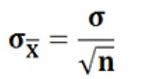
The second value is called the standard error of the mean. A bigger sample gives a narrower sampling distribution. The standard error is the sigma divided by the square root of n, which is why it falls slowly.

Why do We Need the Sampling Distribution of the Sample Mean?

• It is the reference frame for decisions. It shows whether your observed sample mean is common or rare among all possible sample means.
• It sets the width of a confidence interval, through the standard error.
• It powers hypothesis tests. A p value is a tail area of a sampling distribution.
• It explains why bigger samples are better. A larger n makes the distribution narrower.

Sampling Distribution of the Sample Mean Example

The live page: four rowers weigh 154, 158, 162 and 166 lb. List all samples of size 2, with replacement. Find the probability distribution, the mean and the standard deviation of the sample mean.

Step 1: List All 16 Samples

With replacement means that the same rower can be picked twice. There are 4 times 4 = 16 equally likely samples. This table shows the mean of each pair, first pick down the side and second pick across the top.

Compare the live page. It shows (154, 166) as 162, but it is 160. It shows (158, 162) as 164, but it is 160. It shows (158, 166) as 164, but it is 162.

Step 2: The Probability Distribution

There are 7 different sample means. Count how many of the 16 samples give each mean.

The shape is a symmetric triangle, peaked at 160. It already looks like a small bell.

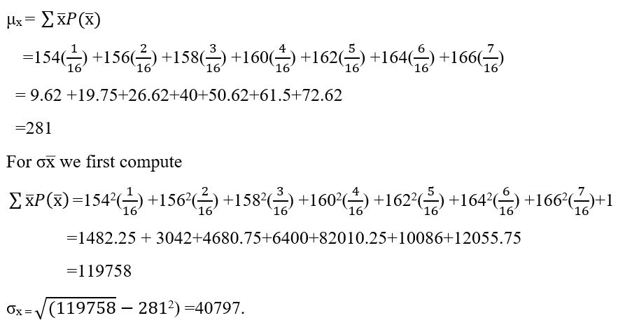
Step 3: Mean and Standard Deviation

• Population mean = (154 + 158 + 162 + 166) divided by 4 = 160 lb.
• Mean of the sample means = 160. It equals the population mean, as the formula says.
• Population sigma = the square root of 20 = 4.4721. The squared gaps from 160 are 36, 4, 4 and 36, which add to 80, and 80 divided by 4 = 20.
• Standard deviation of the sample means = 4.4721 divided by the square root of 2 = 3.1623, which is the square root of 10.

Check by direct calculation from the 16 samples: the standard deviation of the 16 sample means is also 3.1623. The formula and the table agree.

How to Calculate the Sampling Distribution of the Sample Mean?

1. Decide the sample size n and whether you sample with or without replacement.
2. List the possible samples, or simulate many random samples.
3. Find the mean of each sample.
4. Count how often each mean occurs, and convert the counts to probabilities.
5. Find the mean and standard deviation of the sample means, and check them against mu and sigma divided by the square root of n.

The Central Limit Theorem: Why the Shape Becomes Normal

If the population is normal, the sampling distribution of the mean is exactly normal for any sample size. The live page says it is likely to be normal. It is more than likely, it is exact.

If the population is not normal, the central limit theorem takes over: as n grows, the sampling distribution of the mean gets closer to a normal curve. A common rule of thumb is n of 30 or more, but a very skewed population may need more.

To see it, I made a skewed population of 100,000 values, like waiting times, with a mean near 10 and a standard deviation near 10. Then I took 5,000 samples of each size and measured the spread and the skew of the sample means. Skew near 0 means a symmetric shape.

Two things stand out. The spread follows sigma divided by the square root of n very closely. And the skew drops from 1.89 toward 0 as n grows, so the shape becomes a bell even though the population is far from one.

Simulate the Sampling Distribution in Python

I ran the code below, and the output is real.

import itertools
import numpy as np
from collections import Counter
from scipy import stats

# Rowers: weights in lb, samples of size 2 with replacement
w = [154, 158, 162, 166]
pairs = list(itertools.product(w, repeat=2))
means = [sum(p) / 2 for p in pairs]
print("Number of samples:", len(pairs))
for m, k in sorted(Counter(means).items()):
    print("Mean", m, " ways", k, " probability", k, "/16")
print("Mean of sample means:", np.mean(means), " Population mean:", np.mean(w))
print("SD of sample means:", round(float(np.std(means)), 4))
print("Population sigma:", round(float(np.std(w)), 4), " sigma/sqrt(2):", round(float(np.std(w) / 2 ** 0.5), 4))

# Skewed population: sample means look more normal as n grows
rng = np.random.default_rng(5)
pop = rng.exponential(10, 100000)
print("Population mean:", round(float(pop.mean()), 2), " sd:", round(float(pop.std()), 2), " skew:", round(float(stats.skew(pop)), 2))
for n in (1, 5, 30, 100):
    sm = rng.choice(pop, (5000, n)).mean(axis=1)
    print("n", n, " mean of means:", round(float(sm.mean()), 2), " sd:", round(float(sm.std()), 2),
          " formula:", round(float(pop.std() / n ** 0.5), 2), " skew:", round(float(stats.skew(sm)), 2))

Number of samples: 16
Mean 154.0  ways 1  probability 1 /16
Mean 156.0  ways 2  probability 2 /16
Mean 158.0  ways 3  probability 3 /16
Mean 160.0  ways 4  probability 4 /16
Mean 162.0  ways 3  probability 3 /16
Mean 164.0  ways 2  probability 2 /16
Mean 166.0  ways 1  probability 1 /16
Mean of sample means: 160.0  Population mean: 160.0
SD of sample means: 3.1623
Population sigma: 4.4721  sigma/sqrt(2): 3.1623
Population mean: 9.96  sd: 9.95  skew: 1.99
n 1  mean of means: 10.07  sd: 9.86  formula: 9.95  skew: 1.89
n 5  mean of means: 10.08  sd: 4.47  formula: 4.45  skew: 0.8
n 30  mean of means: 9.94  sd: 1.78  formula: 1.82  skew: 0.36
n 100  mean of means: 9.97  sd: 1.01  formula: 1.0  skew: 0.2

Common Mistakes to Avoid

Practice Questions

1. A population has mean 50 and standard deviation 12. For samples of size 36, what are the mean and the standard deviation of the sample mean?
2. The weights are 2, 4 and 6. List the 9 samples of size 2 with replacement, and find the mean of each. What is the mean of the sample means?
3. What happens to the standard deviation of the sample mean if n goes from 25 to 100?
4. Does the sampling distribution of the mean need the population to be normal?

Answers: 1) The mean is 50. The standard deviation is 12 divided by 6 = 2. 2) The means are 2, 3, 4, 3, 4, 5, 4, 5 and 6. Their mean is 36 divided by 9 = 4, which is the population mean. 3) It halves. 4) No. For a large n, the central limit theorem makes it close to normal, but for a small n, you need a normal population. These are my own answers, so please recheck them before publishing.

The sampling distribution of the sample mean is centred on the population mean and has a spread of sigma divided by the square root of n. Once you can build one by hand, as in the rower example, confidence intervals and hypothesis tests stop being formulas and start making sense.