Standard Error of the Mean: Definition, Formula and Worked Examples

You measure the heights of 20 girls in a school and get an average of 150 cm. Measure another 20 and you might get 149. A third group might give 151. None of these is wrong. Each average is a little different because each group is a different sample. The standard error of the mean tells you how much those averages usually move.

It is one of the most used numbers in statistics and one of the most confused. It is not the same as the standard deviation, though people mix them up all the time. It sits behind confidence intervals, margin of error and hypothesis tests, so a clear idea here helps with all of them.

This tutorial explains the definition, the sampling distribution it comes from, the formula and the steps, a worked example with every number, why it shrinks as the sample grows, how it differs from the standard deviation and how to calculate it in Python.

Standard Error of the Mean Definition

The standard error of the mean, often written SEM, is the standard deviation of the sampling distribution of the sample mean. In plain words, it measures how much sample averages vary from sample to sample. A small value means that the sample mean is a precise estimate of the population mean.

The live page calls it a method to estimate the approximate standard deviation of a sampling distribution. It is not a method. It is the measure itself.

What is a Sampling Distribution?

Take many random samples of the same size from one population. Work out the mean of each sample. Plot all those means. The result is the sampling distribution of the sample mean.

The live page explains it as the mean of the population the items come from. That is not right. The sampling distribution is the spread of the sample means across repeated samples. Its centre is near the population mean, and its spread is the standard error.

If the population is normal, the sampling distribution of the mean is exactly normal for any sample size. If the population is not normal, the central limit theorem says that it gets close to normal as the sample grows. The live page says likely, which is too vague.

The School Example

The live page: a school has 1,000 girls, and you want their average height. Take random sets of 20 girls, find each set’s mean (x1 bar, x2 bar and so on up to x20 bar), and look at how those means vary. The page stops there. I finish it in the simulation below.

Standard Error of the Mean Formula

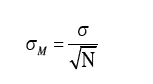
• sigma = the standard deviation of the original population (or the sample standard deviation s, if sigma is unknown).
• n = the sample size.
• Standard error = the standard deviation of the sample means.

The live page uses the capital letter N for the sample size and writes sigma m for the standard error, and gives no formula in text. The formula above is the standard one.

Why do We Need the Standard Error of the Mean?

• Large sample theory. It tells you how fast a sample mean settles near the true mean.
• Confidence intervals. The margin of error is z times the standard error.
• Hypothesis tests. Z and T statistics divide a difference by a standard error.
• Comparing studies. A smaller standard error means a more precise estimate.

Standard Error and Sample Size

The live page says that the standard error is inversely proportional to the sample size. The right statement is that it is inversely proportional to the square root of the sample size. Look at the numbers, with sigma = 8:

Four times the data halves the standard error. To cut it to a tenth, you need a hundred times the data. That is why very large samples bring diminishing returns.

How to Calculate the Standard Error of the Mean?

1. Find the sample mean by adding the values and dividing by n.
2. Find each deviation from the mean, and square it.
3. Add the squared deviations, and divide by n minus 1. This is the sample variance.
4. Take the square root. This is the sample standard deviation, s.
5. Divide s by the square root of n. The result is the standard error.

The live page gives these steps only as an image.

Standard Error of the Mean Example

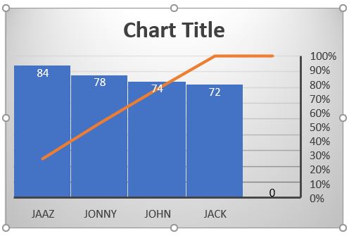
The live page lists the weights of four people: Jack 72 kg, John 74, Jonny 78 and Jazz 84.

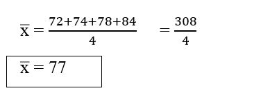
• Mean = (72 + 74 + 78 + 84) divided by 4 = 308 divided by 4 = 77 kg.
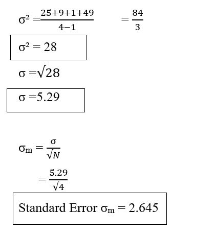
• Sum of squared deviations = 25 + 9 + 1 + 49 = 84.
• Sample variance = 84 divided by 3 = 28.
• Sample standard deviation = the square root of 28 = 5.2915 kg.
• Standard error = 5.2915 divided by the square root of 4 = 2.6458 kg.

Meaning: with only four people, the average of 77 kg could easily be off by about 2.6 kg. The live page calls the mean of the squared deviations the standard deviation. Dividing 84 by 4 gives 21, which is the population variance, and it is a variance, not a standard deviation. The page stops there and never shows a standard error.

Note that this one group of four people gives a single sample mean, so the standard error is estimated from the spread of the people with the formula. In the simulation below, the standard error is measured directly from many sample means.

Standard Error vs Standard Deviation

In the weights example, the standard deviation is 5.29 kg and the standard error is 2.65 kg. The first tells you how much people differ. The second tells you how much the average could be off.

See It in a Simulation

I built a made up school of 1,000 girls with heights near 150 cm and a standard deviation of about 8 cm. I took 20 random sets of 20 girls and measured the spread of their 20 means. Then I repeated it with 5,000 sets. The formula says that the standard error should be 8.01 divided by the square root of 20 = 1.79.

import numpy as np
from scipy import stats

# Page example: weights of four people (kg)
w = np.array([72, 74, 78, 84])
print("Mean:", w.mean(), " Sum of squared deviations:", float(((w - w.mean()) ** 2).sum()))
print("Population variance (divide by n):", float(w.var()), " Sample variance (divide by n-1):", float(w.var(ddof=1)))
sd = w.std(ddof=1)
print("Sample SD:", round(float(sd), 4), " Standard error:", round(float(sd / len(w) ** 0.5), 4))
print("Same with scipy:", round(float(stats.sem(w)), 4))

# Standard error shrinks with the square root of n (sigma = 8)
for n in (5, 20, 80, 320):
    print("n", n, " standard error:", round(8 / n ** 0.5, 3))

# School example: 1000 girls (made up), take 20 random sets of 20
rng = np.random.default_rng(11)
heights = rng.normal(150, 8, 1000)
means = [rng.choice(heights, 20, replace=False).mean() for _ in range(20)]
print("Population sd:", round(float(heights.std()), 2))
print("Sd of 20 sample means:", round(float(np.std(means, ddof=1)), 2), " Formula sigma/sqrt(20):", round(float(heights.std() / 20 ** 0.5), 2))

# Many sets: 5000 samples of 20
means = [rng.choice(heights, 20, replace=False).mean() for _ in range(5000)]
print("Sd of 5000 sample means:", round(float(np.std(means, ddof=1)), 2))

Mean: 77.0  Sum of squared deviations: 84.0
Population variance (divide by n): 21.0  Sample variance (divide by n-1): 28.0
Sample SD: 5.2915  Standard error: 2.6458
Same with scipy: 2.6458
n 5  standard error: 3.578
n 20  standard error: 1.789
n 80  standard error: 0.894
n 320  standard error: 0.447
Population sd: 8.01
Sd of 20 sample means: 1.81  Formula sigma/sqrt(20): 1.79
Sd of 5000 sample means: 1.78

The measured spread of the sample means, 1.81 for 20 sets and 1.78 for 5,000 sets, is very close to the formula value of 1.79. That is the standard error in action.

Standard Error and Confidence Intervals

A 95 percent confidence interval for a mean is the sample mean plus or minus 1.96 standard errors. For the weights data, with the t value for 3 degrees of freedom, the interval is wide because the sample is tiny. With more data the standard error falls, and the interval narrows.

Common Mistakes to Avoid

Practice Questions

1. sigma = 12 and n = 36. Find the standard error.
2. What happens to the standard error if you take 4 times as many samples?
3. A sample of 25 has a standard deviation of 10. Find the standard error of the mean.
4. Is the standard error larger or smaller than the standard deviation (for n above 1)?

Answers: 1) 12 divided by 6 = 2. 2) It halves. 3) 10 divided by 5 = 2. 4) Smaller, since you divide by the square root of n. These are my own answers, so please recheck them before publishing.

The standard error is the bridge from one sample to the whole population. It tells you how far the average can wander, and it shrinks with the square root of the sample size. Report it with every mean, and keep it apart from the standard deviation.