Coefficient of Determination (R Squared): Definition, Formula and Examples

You fit a model that predicts exam scores from hours studied. It gives an answer for every student. But how good is it? One number is used most often to answer that: the coefficient of determination, written R squared. A value of 0.94 means the model explains 94 percent of the ups and downs in scores.

R squared sits at the heart of regression. It is the first number most reports show and the first one that gets misused. People treat a high value as proof that the model is right, or a low value as proof that it is useless. Neither is true and this tutorial shows why.

You will learn what R squared means, its formula in plain steps, a fully worked example, how it links to correlation, what a good value looks like, adjusted R squared, the cases where R squared can be negative, and how to calculate it in Python.

Coefficient of Determination Definition

The coefficient of determination is a statistic that tells you what share of the variation in the outcome is explained by the model. It is written R squared (R2). It is also called a goodness of fit measure.

An R squared of 0.50 means that about half of the observed variation in the outcome is explained by the model. The rest is left unexplained, because of other factors or random noise.

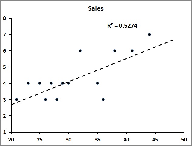
Why do We Need the Coefficient of Determination?

• To judge fit. It shows how closely the model follows the data.
• To compare models on the same data and the same outcome.
• To explain results in simple words: this model explains 94 percent of the variation.
• To track trends. Analysts use it to see how strongly one factor moves with another.

In a simple linear model, R squared equals the square of the correlation coefficient r. If r is 0.97, then R squared is 0.94. A value of 1 is a perfect fit. A value of 0 means that the model does no better than predicting the average every time.

Important: R squared shows association, not cause. The live page says it shows how much variability in one factor another can cause. A model with a high R squared does not show that one thing causes the other.

Coefficient of Determination Formula

• SS residual is the sum of squared errors: add up (actual value minus predicted value) squared, for all points. It is the variation the model fails to explain.
• SS total is the sum of (actual value minus the mean of the actual values) squared. It is the total variation in the outcome.

The fraction SS residual divided by SS total is the share left unexplained. Subtract it from 1 and you get the share explained.

For simple linear regression, there is a shortcut: R squared = r times r.

Coefficient of Determination Example

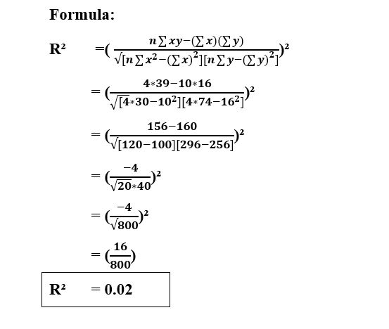
Eight students study 1 to 8 hours and score 52, 55, 61, 60, 68, 72, 70 and 79. The data are made up for teaching.

1. Fit the line. Least squares gives: score = 48.286 + 3.631 times hours.
2. Find SS total. The scores vary around their mean, and the sum of squared differences is 587.88.
3. Find SS residual. The sum of squared gaps between the actual and predicted scores is 34.15.
4. Apply the formula. R squared = 1 minus 34.15 divided by 587.88 = 0.9419.
5. Check with correlation. The correlation r is 0.9705, and 0.9705 squared is 0.9419. The two agree.

Meaning: hours studied explain about 94 percent of the variation in scores. The other 6 percent comes from things the model does not know, such as sleep, past knowledge or luck.

What is a Good R Squared?

There is no single answer. It depends on the field and on the goal.

A high R squared can still go with a bad model. It can come from overfitting, a model that matches the noise in the training data. A low R squared can go with a useful model, when the effect is real but the data are noisy. Always look at residual plots, and test on new data.

Adjusted R Squared

On the training data, R squared never goes down when you add a predictor, even a useless one. So it can reward a model for being bigger, not better. Adjusted R squared corrects for this with a penalty for the number of predictors. Use it when you compare models with different numbers of predictors.

Adjusted R squared = 1 minus (1 minus R squared) times (n minus 1) divided by (n minus k minus 1), where n is the number of observations and k is the number of predictors. In the example, n is 8 and k is 1, which gives 0.9322.

Can R Squared Be Negative?

The live page says that R squared lies between 0 and 1. For a least squares line tested on the data it was fitted to, that is true. But when a model is scored on new data, or when it is not fitted by least squares, SS residual can be larger than SS total, and R squared becomes negative. It means the model is worse than simply predicting the average. In the code below, a model that always predicts 40 for these scores gets R squared of minus 8.25.

Calculate R Squared in Python

I ran the code below, and the output is real.

import numpy as np
from sklearn.linear_model import LinearRegression
from sklearn.metrics import r2_score

# Hours studied vs exam score (made up), 8 students
x = np.array([1, 2, 3, 4, 5, 6, 7, 8])
y = np.array([52, 55, 61, 60, 68, 72, 70, 79])

m = LinearRegression().fit(x.reshape(-1, 1), y)
pred = m.predict(x.reshape(-1, 1))
ss_res = float(((y - pred) ** 2).sum())
ss_tot = float(((y - y.mean()) ** 2).sum())
print("Slope:", round(float(m.coef_[0]), 3), " Intercept:", round(float(m.intercept_), 3))
print("SS_res:", round(ss_res, 2), " SS_tot:", round(ss_tot, 2))
print("R2 by formula:", round(1 - ss_res / ss_tot, 4))
print("R2 by sklearn:", round(r2_score(y, pred), 4))
r = np.corrcoef(x, y)[0, 1]
print("Correlation r:", round(float(r), 4), " r squared:", round(float(r ** 2), 4))

# Adjusted R2 with k = 1 predictor
n, k = len(y), 1
print("Adjusted R2:", round(1 - (1 - r2_score(y, pred)) * (n - 1) / (n - k - 1), 4))

# Predicting the mean only gives R2 = 0
print("R2 of always predicting the mean:", round(r2_score(y, np.full(8, y.mean())), 4))

# A bad model can give a negative R2
print("R2 of a bad model:", round(r2_score(y, np.full(8, 40.0)), 2))

Slope: 3.631  Intercept: 48.286
SS_res: 34.15  SS_tot: 587.88
R2 by formula: 0.9419
R2 by sklearn: 0.9419
Correlation r: 0.9705  r squared: 0.9419
Adjusted R2: 0.9322
R2 of always predicting the mean: 0.0
R2 of a bad model: -8.25

Common Mistakes to Avoid

Practice Questions

1. SS residual is 20 and SS total is 80. What is R squared?
2. The correlation between two variables is 0.8 in a simple linear model. What is R squared?
3. A model has R squared of 0.62. What share of the variation is unexplained?
4. Can R squared be negative? When?

Answers: 1) 1 minus 20 divided by 80 = 0.75. 2) 0.8 times 0.8 = 0.64. 3) 38 percent. 4) Yes, when a model fits worse than the mean, for example on new data. These are my own answers, so please recheck them before publishing.

R squared is a useful first look at a model, not a verdict. Read it as the share of variation explained, pair it with residual checks and new data, and never use it alone to claim that one thing causes another.