T- test Statistics
Introduction to T Test Statistics: Formula, Types and Examples
A class of 25 students scores an average of 90 on an IQ style test, while the national average is 100. Is that class really below average, or did you simply get an unlucky group of 25? A difference in averages is easy to see. Deciding whether it is large enough to matter, given how few people you measured, is what a t test does.
It is one of the most used tests in data science and research. A and B tests, drug trials, quality checks and before and after studies all lean on it. It was designed for exactly the situation that analysts meet every day: a small or medium sample, and no knowledge of the true spread of the population.
This tutorial explains what a t test is, why it exists, how the t score differs from a z score, the three main types with their formulas, three worked examples with real numbers, how to read the result correctly, and how to run it in Python. You should know what a null hypothesis is and what standard deviation measures.
What is the T Test?
A t test is a hypothesis test that uses the t statistic to decide whether to reject a null hypothesis. It compares a sample mean with a target value, or compares two means with each other, and tells you whether the gap is bigger than random sampling variation would usually produce.
The t statistic works like a z score. It measures how many standard errors the sample mean is away from the value in the null hypothesis. The larger its size, the stronger the evidence that the difference is real.
Use a t test when the population standard deviation is unknown, which is nearly always the case in practice, and especially when the sample is small.
Why do We Need the T Test?
Take the bowling example from the live page. A team averages 215, and the average bowler scores 79.9. The team average looks far higher. But if you only watched a handful of games, you would still wonder if it was luck. A t test answers this by weighing the size of the gap against the spread of the scores and the number of games.
Here is a version with the numbers that the page left out. These two numbers are my assumption: 8 bowlers in the team, with a standard deviation of 30. Then:
- The standard error is 30 divided by the square root of 8 = 10.61.
- t = (215 minus 79.9) divided by 10.61 = 12.74, with 7 degrees of freedom.
- The two sided p value is about 0.0000043.
That is very strong evidence that this team is not an average team. A p value that small means the gap would be extremely unlikely if the team were really average. The live page says that a p value under 0.05 means the difference is real, and above it means chance. Better to say this: a small p value means your data would be surprising if the null hypothesis were true, so you doubt the null hypothesis. 0.05 is a common convention, not a law of nature.
A t Value Alone Means Little
Always read the t value together with its degrees of freedom and its p value. The same t of 2 can be significant with a large sample and not significant with a very small one. Also, a significant result does not show that anyone should turn professional. It says the gap is unlikely to be chance. It does not say that the gap is big or useful.
T Score vs Z Score
| Point | Z score and z test | T score and t test |
|---|---|---|
| Population standard deviation | Known | Unknown. Use the sample standard deviation |
| Needs | Population mean, population standard deviation, sample mean, sample size | Population mean (or a second sample), sample mean, sample standard deviation, sample size |
| Distribution | The normal curve | The t distribution, with heavier tails for small samples |
| Typical use | Rare in practice, or with very large samples | Most real analyses |
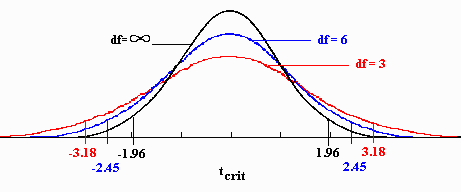
The t distribution has fatter tails than the normal curve when the sample is small, because the sample standard deviation is itself uncertain. That is why the t test demands stronger evidence from small samples. As the sample grows, the t distribution turns into the normal curve. This table shows the critical value for a two sided test at the 0.05 level.
| Degrees of freedom | Critical t value |
|---|---|
| 5 | 2.571 |
| 10 | 2.228 |
| 29 | 2.045 |
| 100 | 1.984 |
| 1000 | 1.962 |
| Normal curve (z) | 1.960 |
The live page says to use a t test when the sample is under 30. That is a rule of thumb. The table shows that there is no sudden jump at 30. The real condition is whether you know the population standard deviation, and if you do not, the t test is right at any sample size.
The Three Types of T Test
| Type | Use it to | Example |
|---|---|---|
| One sample | Compare a sample mean with a known value | Is the class average different from 100? |
| Paired | Compare two measurements on the same people or items | Weight before and after a programme |
| Independent two sample | Compare the means of two separate groups | Marks of two teaching methods |
T Test Statistics Formula
The live page says that there is no single formula. There is one for each type.
Here s is the sample standard deviation and n is the sample size. The bottom part of each formula, s divided by the square root of n, is the standard error.
T Test Statistics Example
Example 1: One Sample T Test, the IQ Class
The live page says the known mean is 100, and the class mean is 90. It gives no sample size, no spread, and no result. I assume 25 students, with a sample standard deviation of 15. These two numbers are my assumption.
- Hypotheses. H0: the class mean is 100. H1: it is not 100.
- Standard error = 15 divided by the square root of 25 = 3.
- t = (90 minus 100) divided by 3 = minus 3.33. Degrees of freedom = 24.
- Compare. The critical value at 0.05 for 24 degrees of freedom is 2.064. The size of minus 3.33 is larger than 2.064.
- p value = 0.0028, which is below 0.05.
Conclusion: we reject the null hypothesis. This class scores lower than 100 by more than chance would normally allow. A 95 percent interval for the class mean runs from 83.81 to 96.19, and it does not contain 100. Note that this applies to this class, and we cannot say why they score lower.
Example 2: Paired T Test, Weight Loss
The live page mentions a weight loss example, with no numbers. Here is one with made up data. Ten people are weighed in kilograms before and after a programme.
| Person | 1 | 2 | 3 | 4 | 5 | 6 | 7 | 8 |
|---|---|---|---|---|---|---|---|---|
| Before | 82 | 91 | 76 | 88 | 95 | 79 | 85 | 90 |
| After | 78 | 88 | 75 | 83 | 90 | 78 | 80 | 86 |
Persons 9 and 10 have before and after weights of 84 and 83, and 87 and 82. The mean loss is 3.4 kg, and the standard deviation of the ten differences is 1.776. The standard error is 1.776 divided by the square root of 10 = 0.562. So t = 3.4 divided by 0.562 = 6.05, with 9 degrees of freedom, and the p value is 0.00019. The loss is very unlikely to be chance. Remember that without a comparison group, the test cannot say that the programme caused it.
Example 3: Two Independent Groups
Two teaching methods are tried on two separate groups of 10 students. Group A marks are 72, 75, 78, 80, 83, 85, 88, 90, 92 and 95, with a mean of 83.8. Group B marks are 65, 68, 70, 72, 74, 75, 78, 80, 82 and 84, with a mean of 74.8. The Welch t test gives t = 2.91 and a p value of 0.0097. The gap of 9 marks is unlikely to be chance. The effect size, Cohens d, is 1.3, which is large.
Report the effect size next to the p value. The p value tells you whether the gap is likely real. The effect size tells you how big it is.
Assumptions of the T Test
- Independent observations. One value does not affect another. For paired tests, the pairs are independent of each other.
- Roughly normal data, or a large enough sample. The test is fairly robust, but very skewed data with a small sample can mislead.
- For the classic two sample test, similar spread in both groups. Welch’s version does not need this, so it is a safer default.
- Continuous data. The values are measurements, such as marks or weights.
Run the T Test in Python
I ran the code below, and the output is real.
In SciPy, ttest_1samp does the one sample test, ttest_rel the paired test and ttest_ind the two sample test. Set equal_var to False for the Welch version.
Common Mistakes to Avoid
| Mistake | Fix |
|---|---|
| Describing the p value as the odds of chance | It is the probability of results at least this extreme if the null hypothesis is true |
| Treating 0.05 as a law | It is a convention. Choose alpha before the test |
| Using an independent test on paired data | Use the paired test for the same people measured twice |
| Ignoring the effect size | Report Cohens d or the mean difference with an interval |
| Running many t tests on many groups | Use ANOVA, or correct for multiple tests |
| Saying not significant proves no difference | The test may lack power |
| Using a t test on categories | Use a chi square test for counts |
Practice Questions
- A sample of 16 has a mean of 52 and a standard deviation of 8. Test against a mean of 50. Find t and the degrees of freedom.
- Which t test should you use to compare the sales of 12 stores before and after a new layout?
- When would you use a z test instead of a t test?
- A t test gives p = 0.03 at alpha 0.05. What is your decision?
Answers: 1) Standard error = 8 divided by 4 = 2, t = (52 minus 50) divided by 2 = 1.0, degrees of freedom = 15. 2) A paired t test, since the same stores are measured twice. 3) When the population standard deviation is known. 4) Reject the null hypothesis, since 0.03 is below 0.05. These are my own answers, so please recheck them before publishing.
A t test boils a comparison down to a clear question: is this gap bigger than the noise in my data would explain? Pick the right type, check the assumptions, read the p value with the effect size, and keep in mind that the test tells you about a gap and not about its cause.
